
arxiv: Conservative Q-Learning for Offline Reinforcement Learning
作者的代码:CQL-Github
Effectively leveraging large, previously collected datasets in reinforcement learn- ing (RL) is a key challenge for large-scale real-world applications. Offline RL algorithms promise to learn effective policies from previously-collected, static datasets without further interaction. However, in practice, offline RL presents a major challenge, and standard off-policy RL methods can fail due to overestimation of values induced by the distributional shift between the dataset and the learned policy, especially when training on complex and multi-modal data distributions.
如何在强化学习(RL)中有效利用以前收集的大型数据集是大规模在现实世界应用所面临的关键挑战。离线RL算法允许了从以前收集的静态数据集中学习有效的策略,而无需与环境交互。然而,在实践中,离线RL一个主要的挑战是:标准的off-policy RL算法可能会因为数据集和学习策略之间的 distributional shift 导致V值估计过高而失效,尤其是在对复杂和多模态数据分布进行训练时。
In this paper, we propose conservative Q-learning (CQL), which aims to address these limitations by learning a conservative Q-function such that the expected value of a policy under this Q-function lower-bounds its true value. … If we can instead learn a conservative estimate of the value function, which provides a lower bound on the true values, this overestimation problem could be addressed.
Aviral Kumar等人提出了保守Q学习(CQL),其目的是通过学习一个保守的Q函数来解决这些限制,使得在该Q函数下策略的期望值低于其真实值。 …… 如果我们能够学习值函数的保守估计,它反映了真实Q值的下界,那么这个高估问题就可以得到解决。
In practice, CQL augments the standard Bellman error objective with a simple Q-value regularizer which is straightforward to implement on top of existing deep Q-learning and actor-critic implementations.
在实践中,CQL用一个简单的Q值正则化项增强了Bellman error objective的性能,这个修改在现有的deep Q-learning和Actor-Critic算法基础之上都很易于实现。(只需修改大概20行代码)
Directly utilizing existing value-based off-policy RL algorithms in an offline setting generally results in poor performance, due to issues with bootstrapping from out-of-distribution actions and overfitting. If we can instead learn a conservative estimate of the value function, which provides a lower bound on the true values, this overestimation problem could be addressed.
在离线强化学习环境中直接使用现有的基于值的 off-policy 算法通常会导致较差的性能,这是由于OOD的actions 评估(源于收集数据的策略和学习的策略之间的distributional shift)和自举带来的过拟合问题。如果我们能够学习值函数的保守估计(真值下界),那么这个高估问题就可以得到解决。
In fact, because policy evaluation and improvement typically only use the value of the policy, we can learn a less conservative lower bound Q-function, such that only the expected value of Q-function under the policy is lower-bounded, as opposed to a point-wise lower bound.
因为实际上策略评估和改进通常只使用策略的值,所以我们可以学习一个不太保守的Q函数下界,这样该策略下Q函数是期望意义上的下界,而不是逐点的下界(允许某些点不是下界)。
the key idea behind our method is to minimize values under an appropriately chosen distribution over state-action tuples, and then further tighten this bound by also incorporating a maximization term over the data distribution.
我们的方法背后的关键思想是在适当的一些状态-动作组 (s,a) (数据集外的)上最小化值,然后再通过在引入最大化项(在数据集内的)来进一步收紧这一界限。
Preliminaries
The goal in reinforcement learning is to learn a policy that maximizes the expected cumulative discounted reward in a Markov decision process (MDP)。
强化学习的目标是在马尔可夫决策过程(MDP)中学习使预期累积折扣回报最大化的策略。
D is the dataset, and is the discounted marginal state-distribution of .
边际先验分布(Marginal Prior Distribution)是在没有考虑其他参数的条件下对单个参数的分布进行建模。具体来说,假设我们有一个参数向量θ,其中包含多个参数。边际先验分布是指我们只对其中一些参数感兴趣,而对其他参数不关心。因此,通过将其他参数积分或边际化掉,我们得到一个边际先验分布,其中包含我们关心的参数。
如果对于论文和文章中的符号有不明白的,请参阅这篇文章CQL1(下界Q值估计)
Off-policy RL algorithms based on dynamic programming maintain a parametric Q-function and, optionally, a parametric policy, . Q-learning methods train the Q-function by iteratively applying the Bellman optimality operator.
基于动态规划的Off-policy 算法保持参数Q函数 ,以及可选的参数策略 。
Q学习方法通过迭代应用Bellman最优算子来训练Q函数。
Bellman 最优算子(QL)与Bellman算子(AC)
Bellman 最优算子为Q-Learning(QL)更新时候采用的Q值更新方式,称之为,定义如下,其中 γ 为折扣因子(discounted-factor):
Bellman算子为Actor-Critic(AC)更新时候采用的Q值更新方式,称之为,定义如下:
In an actor-critic algorithm, a separate policy is trained to maximize the Q-value. Actor-critic methods alternate between computing via (partial) policy evaluation, by iterating the Bellman operator , where is the transition matrix coupled with the policy, and improving the policy π(a|s) by updating it towards actions that maximize the expected Q-value.
在Actor-Critic算法中,训练单独的策略以最大化Q值。Actor-critic方法在通过(部分)策略评估计算之间交替,方法是迭代Bellman算子(其中是与策略耦合的状态转换矩阵),以及改进策略π(a|s),更新以最大化期望Q值。
第一行中的方程等价于以下方程,证明:link
但是显然的在Offline RL中存在这样的问题,上述公式中的 r(s,a) 在Offline中是无法获取的,Since无法与环境进行探索,策略 π 被由于价值最大化操作,价值估计很可能就会偏向于错误的高Q值的 out-of-distribution (OOD) 行为。
The Conservative Q-Learning (CQL) Framework
离线强化学习面对的巨大挑战是如何减少外推误差。实验证明,外推误差主要会导致在远离数据集的点上Q函数的过高估计,甚至常常出现Q值向上发散的情况。因此,如果能用某种方法将算法中偏离数据集的点上的Q函数保持在很低的值,或许能消除部分外推误差的影响,这就是保守 Q-learning(conservative Q-learning,CQL)算法的基本思想。CQL 在普通的贝尔曼方程上引入一些额外的限制项,达到了这一目标。
develop a conservative Q-learning algorithm, such that the expected value of a policy under the learned Q-function lower-bounds its true value(真实Q值函数下界). Lower-bounded Q-values prevent the over-estimation that is common in offline RL settings due to OOD actions and function approximation error.
CQL算法使策略在所学习的Q函数的期望值低于其 真值(真实Q值函数下界)。Q值函数下界防止了由于OOD动作和函数近似误差而在 offline RL 环境中常见的过度估计。
Conservative Off-Policy Evaluation
普通 DQN 类方法通过优化 stander Bellman error objective 来更新 Q 价值
Because we are interested in preventing overestimation of the policy value, we learn a conservative, lower-bound Q-function by additionally minimizing Q-values alongside a standard Bellman error objective. Our choice of penalty is to minimize the expected Q-value under a particular distribution of state-action pairs, µ(s, a).
由于我们想要预防高估价值函数,我们可以通过在保留 标准的 Bellman error objective 的同时,额外最小化Q值来学习保守的Q函数下界。我们选择的惩罚项是希望在某个特定分布µ(s, a)上的期望Q值最小。
又考虑到 的计算中 ,都在 D 中,只有 a’ 是生成的可能 OOD,因此我们限制 中的 s 边缘分布为 ,从而有,迭代更新过程可以表示为:Equation 1
是平衡因子,用来控制两个优化目标的比重。
论文中Theorem 3.1 证明了对任意 ,当 足够大时,迭代的收敛结果 会对每一个状态动作对 都形成真实值的下界,即 。[这里是point-wise的下界]
we can substantially tighten this bound if we are only interested in estimating . If we only require that the expected value of the under π(a|s) lower-bound , we can improve the bound by introducing an additional Q-value maximization term under the data distribution, , resulting in the iterative update (changes in red):
为了防止过于保守,如果我们只对估计只要求关于策略的期望感兴趣,我们可以大大收紧这个界(放松对Q的约束,也就是期望意义上的下界,允许某些点不是下界)。对于符合用于生成数据集 的行为策略 π 的数据点,我们可以认为对这些点的估值较为准确,在这些点上不必限制让值很小,我们可以通过引入对在数据集分布上的Q值进行最大化的项来改进(最小化负值=最大化原值),从而得出(红色标记变化):Equation 2
其中 是利用数据集 得到的对真实行为策略 的估计,因为我们无法获知真实的行为策略,只能通过数据集中已有的数据近似得到。
所以那些在行为策略当中的动作就有可能被高估。
论文中Theorem 3.2 证明了当 时,上式迭代收敛得到的 函数虽然不是在每一点上都小于真实值,但其期望是小于真实值的,即 。[这里不是point-wise的下界]
In summary, we showed that the basic CQL evaluation in Equation 1 learns a Q-function that lower-bounds the true Q-function Qπ , and the evaluation in Equation 2 provides a tighter lower bound on the expected Q-value of the policy π.
总之,我们发现Equation 1中的基本CQL评估学习了一个Q函数,该Q函数下界为真实Q函数,而Equation2的评估为策略π的预期Q值提供了一个更严格的下界。
Conservative Q-Learning for Offline RL
We now present a general approach for offline policy learning, which we refer to as conservative Q-learning (CQL). As discussed in Section 3.1, we can obtain Q-values that lower-bound the value of a policy π by solving Equation 2 with µ = π. How should we utilize this for policy optimization? We could alternate between performing full off-policy evaluation for each policy iterate, , and one step of policy improvement. However, this can be computationally expensive. Alternatively, since the policy is typically derived from the Q-function, we could instead choose µ(a|s) to approximate the policy that would maximize the current Q-function iterate, thus giving rise to an online algorithm.
至此,我们提出了一种离线策略学习的通用方法,称为 保守Q学习(CQL)。但仍有一个缺陷:计算的时间开销太大了。
上面提到,我们可以通过求解Equation 2(其中µ = π)来获得Q值,这些Q值构成了策略π的价值的下界。我们应该如何利用这一点进行策略优化呢?当令 时,迭代的每一步,算法都要对策略 做完整的离线策略评估(迭代以上更新式至收敛)来计算 ,再进行一次策略迭代,而离线策略评估是非常耗时的。作为替代,考虑到策略通常是从在每轮迭代过程中由使 Q 最大的动作中派生出来的,我们可以选择µ(a|s)来近似 将使当前Q函数迭代最大化的 策略,从而产生一种在线算法。
We can formally capture such online algorithms by defining a family of optimization problems over µ(a|s), presented below, with modifications from Equation 2 marked in red. An instance of this family is denoted by CQL(R) and is characterized by a particular choice of regularizer R(µ):
我们可以通过在µ(a|s)上定义一族优化问题来形式化地捕捉这种在线算法,如下所示,下面通过红色标记出来对Equation 2进行的修改。这个被称为CQL(R),为了防止过拟合,再加上正则化项 :Equation 3
Variants of CQL
To demonstrate the generality of the CQL family of optimization problems, we discuss two specific instances within this family that are of special interest, and we evaluate them empirically in Section 6. If we choose to be the KL-divergence against a prior distribution, , i.e., , then we get (for a derivation, see Appendix A). First, if , then the first term in Equation 3 corresponds to a soft-maximum of the Q-values at any states and gives rise to the following variant of Equation 3, called CQL(H):
……如果我们将正则化项采用为对先验策略和 的 KL散度,即,那么我们可以得到。如果取 为均匀分布 ,即 ,那么Equation 3中的第一项对应于任意状态s处Q值的软最大值,并引出以下 CQL(R) 的变体,称为CQL(H):Equation 4
可以注意到,简化后式中已经不含有 µ,为计算提供了很大方便。
详细推导过程请参见 动手做强化学习
论文中 Theorem 3.3 证明了:若策略梯度更新的非常缓慢(足够小的速度更新),不考虑采样误差,即,那么选取,可以保证在迭代更新中的每一步时,都有
论文中 Theorem 3.4 证明了:CQL是gap-expanding的,即对于任意一次迭代,in-distribution动作分布与OOD动作分布产生的Q函数()的差将比在真实Q函数上产生的差更大,公式表达是。本文的方法存在潜在的优势是能够在真实Q函数上缩紧 训练的策略 与行为策略 的差距。换句话表示就是,学习到的策略和行为策略之间的正则化Q函数期望估值差异,都比原本的Q函数大。这样的话在面对函数近似以及采样误差的时候可以更稳定。直观来说就是分布内动作受到分布外动作的影响更小。
Second, if ρ(a|s) is chosen to be the previous policy , the first term in Equation 4 is replaced by an exponential weighted average of Q-values of actions from the chosen πˆ k−1 (a|s). Empirically, we 4 find that this variant can be more stable with high-dimensional action spaces (e.g., Table 2) where it is challenging to estimate via sampling due to high variance. In Appendix A, we discuss an additional variant of CQL, drawing connections to distributionally robust optimization. We will discuss a practical instantiation of a CQL deep RL algorithm in Section 4. CQL can be instantiated as either a Q-learning algorithm (with instead of in Equations 3, 4) or as an actor-critic algorithm.
在实验中,由于高方差,要通过采样估计estimate 并不容易。如果选择ρ(a|s)为先前的策略,那么Equation 4中的第一项将被从选择的的动作的Q值的指数加权平均值所替代。根据实验,这个变种在高维动作空间中可以更加稳定。请见 CQL论文 附录A CQL(var)部分。
CQL可以作为Q学习算法(在Equation 3、4中使用而不是)或作为演员-评论家算法来实现。
Computing
uses log-sum-exp in the objective for training the Q-function (Equation 4). In discrete action domains, we compute the log-sum-exp exactly by invoking the standard tf.reduce_logsumexp() (or torch.logsumexp()) functions provided by autodiff libraries. In continuous action tasks, uses importance sampling to compute this quantity, where in practice, we sampled 10 action samples each at every state s from a uniform-at-random Unif(a) and the current policy, π(a|s) and used these alongside importance sampling to compute it as follows using N = 10 action samples:
在训练Q函数(Equation 4)时在目标函数中使用了 log-sum-exp。在离散动作空间中,我们可以通过调用自动微分库提供的标准函数(tf.reduce_logsumexp()或torch.logsumexp())来精确计算log-sum-exp。在连续动作任务中, 使用重要性采样来计算这个值,在实践中,我们从均匀随机分布Unif(a)和当前策略π(a|s)中对每个状态s采样了10个动作样本,并使用重要性采样来计算如下,其中N = 10表示动作样本的数量:
CQL 代码实践
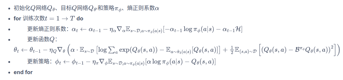
Pseudocode
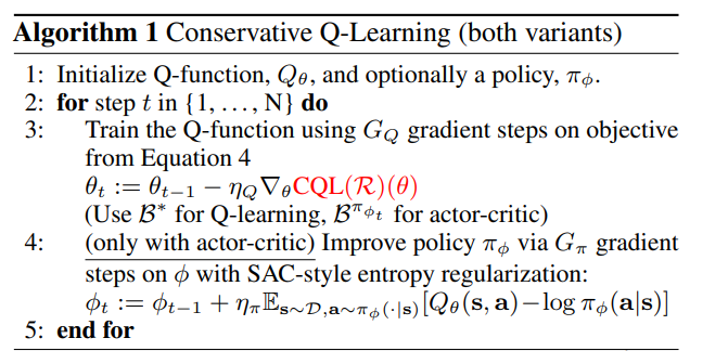
如果是Q-learning模式:μ 可以作为最终的策略 如果是Actor-Critic模式:需要使用SAC的训练方式额外训练actor
动手做强化学习中,CQL代码实践,相较于SAC代码实践主要多的是这一部分:
# 以上与SAC相同,以下Q网络更新是CQL的额外部分
batch_size = states.shape[0]
random_unif_actions = torch.rand([batch_size * self.num_random, actions.shape[-1]],
dtype=torch.float).uniform_(-1, 1).to(device)
random_unif_log_pi = np.log(0.5**next_actions.shape[-1])
print('random_unif_log_pi: ',random_unif_log_pi,np.log(0.5))
tmp_states = states.unsqueeze(1).repeat(1, self.num_random,1).view(-1, states.shape[-1])
tmp_next_states = next_states.unsqueeze(1).repeat(1, self.num_random, 1).view(-1, next_states.shape[-1])
random_curr_actions, random_curr_log_pi = self.actor(tmp_states)
random_next_actions, random_next_log_pi = self.actor(tmp_next_states)
q1_unif = self.critic_1(tmp_states, random_unif_actions).view(-1, self.num_random, 1)
q2_unif = self.critic_2(tmp_states, random_unif_actions).view(-1, self.num_random, 1)
q1_curr = self.critic_1(tmp_states, random_curr_actions).view(-1, self.num_random, 1)
q2_curr = self.critic_2(tmp_states, random_curr_actions).view(-1, self.num_random, 1)
q1_next = self.critic_1(tmp_states, random_next_actions).view(-1, self.num_random, 1)
q2_next = self.critic_2(tmp_states, random_next_actions).view(-1, self.num_random, 1)
q1_cat = torch.cat([
	q1_unif - random_unif_log_pi,
	q1_curr - random_curr_log_pi.detach().view(-1, self.num_random, 1),
	q1_next - random_next_log_pi.detach().view(-1, self.num_random, 1)
	],dim=1)
q2_cat = torch.cat([
	q2_unif - random_unif_log_pi,
	q2_curr - random_curr_log_pi.detach().view(-1, self.num_random, 1),
	q2_next - random_next_log_pi.detach().view(-1, self.num_random, 1)
	],dim=1)

qf1_loss_1 = torch.logsumexp(q1_cat, dim=1).mean()
qf2_loss_1 = torch.logsumexp(q2_cat, dim=1).mean()
qf1_loss_2 = self.critic_1(states, actions).mean()
qf2_loss_2 = self.critic_2(states, actions).mean()
qf1_loss = critic_1_loss + self.beta * (qf1_loss_1 - qf1_loss_2)
qf2_loss = critic_2_loss + self.beta * (qf2_loss_1 - qf2_loss_2)beta是CQL损失函数中的系数,num_random 是CQL中的动作采样数。
上面这段代码的意义是:
-
生成一个随机动作
random_unif_actions,其形状与输入动作actions相同,但是值是在区间[-1, 1]内均匀分布的随机数。random_unif_actions: torch.Size([320, 1]) -
计算一个常数
random_unif_log_pi,它是以 0.5 为底的next_actions张量的维度数的对数。random_unif_log_pi: int -
对输入状态
states和next_states进行扩展,以便与random_unif_actions的维度匹配,从而得到tmp_states和tmp_next_states。tmp_states: torch.Size([320, 3])
这段代码的作用是将states张量进行重复和重新形状操作:states.unsqueeze(1):在维度1上添加一个维度,这样做是为了在后续操作中能够正确地重复states张量。torch.Size([64, 1, 3]).repeat(1, self.num_random, 1):将states张量在维度1上重复self.num_random次(动作采样数),即,得到形状为(batch_size, self.num_random)的张量。这样做是为了在后续操作中生成多个重复的状态。torch.Size([64, 5, 3]).view(-1, states.shape[-1]):将张量重新形状为(batch_size * self.num_random / 3, 3),其中-1表示自动计算该维度的大小。这样做是为了将重复的状态展平为一个二维张量,以便进行后续处理。
-
使用
self.actor函数计算tmp_states和tmp_next_states对应的随机动作以及它们的对数概率。random_curr_actions, random_curr_log_pi: torch.Size([320, 1])此处的states来自于训练集(buffer)中,将该state输入到actor中,因为是连续的动作值,通过高斯分布采样得到random_curr_actions, 以及可以得到对应的log_pi。 -
现在我们就到了采样的action以及对应的log_prob,分别来自于均匀分布、当前s的高斯分布以及下一个s的高斯分布。我们下一步需要得到Q(s,a),也就是需要限制的q。得到的(s,a) 对输入到critic中就行了。使用
self.critic_1和self.critic_2函数计算tmp_states和随机动作random_unif_actions、random_curr_actions、random_next_actions对应的 Q 值。q1: torch.Size([64, 5, 1]) -
将 Q 值按照一定的方式进行组合,得到
q1_cat和q2_cat。这些组合包括将随机动作的 Q 值减去对应的对数概率,并将其与其他 Q 值拼接在一起。q_cat: torch.Size([64, 15, 1]) -
计算
qf_loss_1:将q_cat指数之和的对数压缩到一维(torch.Size([64, 1]),再求平均。这样就构成了:
critic_1_loss是 ,self.beta是公式中的 ,qf1_loss_1 - qf1_loss_2即是 。
| 变量名 | 意义 | 来源 | Size |
|---|---|---|---|
| states | 状态 | Replay Buffer | [64, 3] |
| batch_size | 批次大小 | states | 64 |
| random_unif_actions | 随机均匀采样的动作 | torch.rand().uniform_(-1, 1) | [64*5, 1] |
| random_unif_log_pi | 均匀分布的对数概率 | np.log(0.5) | numpy.float64 |
| tmp_states | 扩展后的状态 | states | [320, 3] |
| tmp_next_states | 扩展后的下一个状态 | next_states | [320, 3] |
| random_curr_actions | 当前动作 | tmp_states | [320, 1] |
| random_curr_log_pi | 当前动作的对数概率 | tmp_states | [320, 1] |
| random_next_actions | 下一个动作 | tmp_next_states | [320, 1] |
| random_next_log_pi | 下一个动作的对数概率 | tmp_next_states | [320, 1] |
| q1_unif / q2_unif | 使用随机均匀采样动作计算Critic的的Q值 | tmp_states, random_unif_actions | [64, 5, 1] |
| q1_curr / q2_curr | 使用随机当前动作计算的第一个Critic的Q值 | tmp_states, random_curr_actions | [64, 5, 1] |
| q1_next / q2_next | 使用随机下一个动作计算的Critic的Q值 | tmp_states, random_next_actions | [64, 5, 1] |
| q1_cat / q2_cat | 拼接后的Critic的Q值 | … | [64, 15, 1] |
| qf1_loss_1 / qf2_loss_1 | Critic的损失函数(q_cat的对数求和的平均值) | q1_cat / q2_cat | FloatTensor |
| qf1_loss_2 / qf2_loss_2 | Critic的损失函数(使用原始状态和动作计算的Q值的平均值) | states, actions | FloatTensor |
| qf1_loss / qf2_loss | Critic的总损失函数 | critic_1_loss + beta * (qf1_loss_1 - qf1_loss_2) | FloatTensor |
Reference:
- Conservative Q-Learning(CQL)保守Q学习(一)-CQL1(下界Q值估计)
- Conservative Q-Learning(CQL)保守Q学习(二)-CQL2(下界V值估计),CQL(R)与CQL(H)(这两篇理论证明过程很详细,缺少对后几个Theorem的详细解释)
- 论文速览【Offline RL】—— 【CQL】Conservative Q-Learning for Offline Reinforcement Learning(很精简)
- CQL: Conservative Q-Learning for Offline Reinforcement Learning (解释很均衡)
- 强化学习 | CQL:Conservative Q-Learning for Offline Reinforcement Learning(这篇对几个Theorem解释较好)
- Conservative Q Learning(保守强化学习)傻瓜级讲解和落地教程
- 【论文笔记】Conservative Q-Learning