
Arxiv: MOPO: Model-based Offline Policy Optimization
PDF: arxiv.org
Code: paperswithcode
Abstract
离线强化学习指的是完全从一批先前收集的数据集中学习策略的问题。尽管model-free 离线RL算法取得了显著进展,但最成功的现有方法将策略限制在数据支持范围内,无法推广到新状态。 MOPO作者观察到,与model-free 算法相比,现有的model-based的RL算法本身已经在离线环境中有显著的优势,尽管它并不是为这种设置而设计的。然而,尽管许多基于标准模型的RL算法已经估计了模型的不确定性,但它们本身并没有提供明确的机制来避免离线设置中的分布偏移问题。因此,作者建议修改现有的model-based的RL算法,以通过将 model-free 离线RL 转换为受惩罚的MDP框架来解决这些问题。 作者从理论上表明,通过使用这种算法,可以使真实MDP下的 奖励的下界 最大化。基于上述理论结果,作者提出了一种新的model-based的离线RL算法,该算法将动力学模型的不确定性作为对奖励函数的惩罚。实验表明,该算法的性能在离线RL benchmark 测试和两项 具有挑战性的 需要对分布外泛化的 连续控制任务中优于现有的model-based 和 model-free RL算法。
Introduction
目前主流的offline RL的方法都是model-free的,这类方法通常需要将策略 π 限制到数据集覆盖的集合范围里(support),不能泛化到没见过的状态上。作者提出MOPO算法,MOPO是一种model-based offline RL方法,简单来说就是把MBPO用在了offline设定下,根据offline的需要做了一些小修改。
一方面,这种model-based方法对环境进行建模,拟合环境的动力学模型(dynamics model),采样效率较高;另一方面,MOPO能够利用model让策略以一定概率选择行为分布之外的action。但是离行为分布越远,不确定性会越大,所以MOPO通过不确定性估计来量化偏离行为分布的风险,实现其和探索多样state所得收益之间的trade-off。具体来说,就是在reward函数后面加了一个不确定性惩罚项,通过ensemble的方法(即N个dynamics模型的最大标准差)量化这种不确定性,不确定性越大则reward越小。也就是说不是直接惩罚OOD状态和动作,而是惩罚具有高不确定性的 (s,a) 。具体做法就是,先根据data去学一堆状态转移函数,这个函数是一个用神经网络表示的关于状态和reward的高斯分布。
While these methods achieve reasonable performances in some settings, their learning is limited to behaviors within the data manifold. Specifically, these methods estimate error with respect to out-of-distribution actions, but only consider states that lie within the offline dataset and do not consider those that are out-of-distribution. We argue that it is important for an offline RL algorithm to be equipped with the ability to leave the data support to learn a better policy for two reasons: (1) the provided batch dataset is usually sub-optimal in terms of both the states and actions covered by the dataset, and (2) the target task can be different from the tasks performed in the batch data for various reasons, e.g., because data is not available or hard to collect for the target task. Hence, the central question that this work is trying to answer is: can we develop an offline RL algorithm that generalizes beyond the state and action support of the offline data?
Model-free 的算法在一些环境下可以达到合理的性能,但它们的学习仅限于数据集内的行为。具体而言,这些方法会针对超出分布的动作估计误差,但只考虑那些在离线数据集中的状态,并不考虑那些超出分布范围的状态。
作者认为,离线RL算法具备离开数据支持范围的能力对于两个原因非常重要:
- 提供的数据集通常在覆盖的状态和动作方面是次优的;
- 目标任务可能由于各种原因与数据集中执行的任务不同。例如,由于目标任务的数据不可用或难以收集。
因此,本文试图回答的核心问题是:我们能否开发一种离线RL算法,可以在超出离据集的状态和动作支持范围之外进行泛化?
To approach this question, we first hypothesize that model-based RL methods make a natural choice for enabling generalization, for a number of reasons. First, model-based RL algorithms effectively receive more supervision, since the model is trained on every transition, even in sparse-reward settings. Second, they are trained with supervised learning, which provides more stable and less noisy gradients than bootstrapping. Lastly, uncertainty estimation techniques, such as bootstrap ensembles, are well developed for supervised learning methods and are known to perform poorly for value-based RL methods.
为了回答这个问题,我们首先假设模型驱动的强化学习(RL)方法在实现泛化方面具有自然优势,原因如下
- model-based RL算法能够更有效地进行监督学习,因为模型在每个transition中都接受训练,即使在稀疏奖励的情况下也是如此。
- 它们通过监督学习进行训练,这提供了比自举法更稳定且噪声更少的梯度。
- 不确定性估计技术(例如Bootstrap ensembles)在监督学习方法中得到了充分发展,而在基于值的RL方法中已知表现不佳。
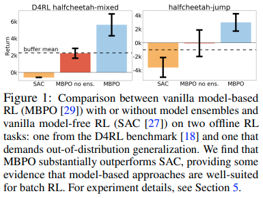
All of these attributes have the potential to improve or control generalization. As a proof-of-concept experiment, we evaluate two state-of-the-art off-policy model-based and model-free algorithms, MBPO and SAC, in Figure 1. Although neither method is designed for the batch setting, we find that the model-based method and its variant without ensembles show surprisingly large gains. This finding corroborates our hypothesis, suggesting that model-based methods are particularly well-suited for the batch setting, motivating their use in this paper.
所有这些特性都有潜力 改善或控制 泛化。作为一个概念验证实验,我们在下图中评估了两种最先进的off-policy model-based和model-free算法,MBPO和SAC。尽管这两种方法都不是为离线强化学习而设计的,但我们发现model-based算法及其不使用 ensemble 的变体都显示出能令人惊讶的巨大增益。这一发现支持了我们的假设,表明model-based算法特别适合于离线环境,并激发了我们在本文中使用它们的动机。
Despite these promising preliminary results, we expect significant headroom for improvement. In particular, because offline model-based algorithms cannot improve the dynamics model using additional experience, we expect that such algorithms require careful use of the model in regions outside of the data support. Quantifying the risk imposed by imperfect dynamics and appropriately trading off that risk with the return is a key ingredient towards building a strong offline model-based RL algorithm. To do so, we modify MBPO to incorporate a reward penalty based on an estimate of the model error. Crucially, this estimate is model-dependent, and does not necessarily penalize all out-of-distribution states and actions equally, but rather prescribes penalties based on the estimated magnitude of model error. Further, this estimation is done both on states and actions, allowing generalization to both, in contrast to model-free approaches that only reason about uncertainty with respect to actions.
尽管有这些令人鼓舞的初步结果,但我们预计还有很大的改进空间。特别是,由于离线model-based算法无法使用额外的经验来改进动力学模型,因此我们认为此类算法需要在数据支持之外的区域谨慎使用模型。量化 不完美的动力学模型 带来的风险,并适当地将风险与回报进行权衡,是构建强大的离线model-based RL算法的关键因素。为此,我们修改了 MBPO,加入了基于模型误差估计的奖励函数惩罚项。至关重要的是,此估计依赖于模型,并且不一定平等地 惩罚 所有的 OOD 状态和操作,而是根据估计的模型误差的大小制定惩罚。此外,这种估计是针对状态和动作进行的,允许对两者进行泛化,这与仅评估动作不确定性的model-free方法形成鲜明对比。
we develop a practical method that estimates model error using the predicted variance of a learned model, uses this uncertainty estimate as a reward penalty, and trains a policy using MBPO in this uncertainty-penalized MDP.
算法使用 学习的模型的预测方差 来估计 模型误差,将这种不确定性估计用作 奖励的惩罚项,并在这种不确定性惩罚的MDP中使用MBPO训练策略。
Uncertainty quantification, a key ingredient to our approach, is critical to good performance in model-based RL both theoretically and empirically, and in optimal control. Unlike these works, we develop and leverage proper uncertainty estimates that particularly suit the offline setting.
不确定性量化是我们方法的关键要素,在理论上和实证上都已经说明了它对于model-based RL和最优控制的性能至关重要。不一样的是,我们需要开发和利用适合离线环境的正确的不确定性估计。
强化学习中的dynamics是什么意思?^安道龙的回答 - 知乎
- Dynamics,动力学,动力学模式,动力学模型
- 该词主要出现在强化学习的Model-base类论文中。
- 指的是,在强化学习中,环境实际的运行机制不叫做模型,而叫做环境动力学(dynamics of environment),它能够明确确定Agent下一个状态和所得的即时奖励。
- 所以动力学指的就是环境运转的动态机制,能够给出状态转移函数和奖励。
- 然后Model-Based的强化学习就是要基于交互信息学习一个环境动力学模型(Dynamics Model),并利用该模型进行辅助训练。
为表述统一方便,这里 dynamics 统一译为 动力学模型。
Related Work
请参考MOPO-Model-based Offline Policy Optimization - betray12138
Preliminaries
| Symbol | Meaning in English | Meaning |
|---|---|---|
| Markov decision process | 马尔可夫决策过程 | |
| state space | 状态空间 | |
| action space | 动作空间 | |
| transition dynamics | 转移函数 | |
| r(s, a) | reward function | 奖励函数 |
| initial state distribution | 初始状态分布 | |
| γ | discount factor | 折扣因子 |
| π(a \mid s) | policy | 策略 |
| expected discounted return | 预测的总奖励函数 | |
| value function | 价值函数 | |
| static dataset | 静态数据集 | |
| behavior policies | 行为策略 | |
| the real dynamics | 真实的动态学模型 | |
| dynamics model, the learned dynamics | 学习的动态学模型,根据估计转移模型 | |
| the probability of being in state s at time step t if actions are sampled according to π and transitions according to | 动态学模型下采取策略π使得智能体在时刻t状态为s的概率 | |
| discounted occupancy measure of policy π under dynamics | 占用度量,动作状态对被访问到的概率 | |
| a model of the transition distribution | 用参数θ表示的状态转移模型 | |
| measures the difference between M and Mc under the test function V π | 在 下衡量了 和 之间的差异 |
MOPO: Model-Based Offline Policy Optimization
our goal is to design an offline model-based reinforcement learning algorithm that can take actions that are not strictly within the support of the behavioral distribution. Using a model gives us the potential to do so. However, models will become increasingly inaccurate further from the behavioral distribution, and vanilla model-based policy optimization algorithms may exploit these regions where the model is inaccurate. This concern is especially important in the offline setting, where mistakes in the dynamics will not be corrected with additional data collection.
我们的目标是设计一种离线model-based RL算法,可以采取 不严格地包含在行为分布(产生的) 的动作。使用模型给予了我们这么做的潜力。然而,模型在远离行为分布的地方会变得越来越不准确,而传统的 model-based 策略优化算法可能会利用这些模型不准确的区域。在离线环境中,这个问题就尤为重要,因为动力学模型的错误不会有额外的数据收集来进行纠正。
For the algorithm to perform reliably, it’s crucial to balance the return and risk: 1. the potential gain in performance by escaping the behavioral distribution and finding a better policy, and 2. the risk of overfitting to the errors of the dynamics at regions far away from the behavioral distribution. To achieve the optimal balance, we first bound the return from below by the return of a constructed model MDP penalized by the uncertainty of the dynamics (Section 4.1). Then we maximize the conservative estimation of the return by an off-the-shelf reinforcement learning algorithm, which gives MOPO, a generic model-based off-policy algorithm (Section 4.2). We discuss important practical implementation details in Section 4.3.
为了使算法能够可靠地运行,平衡回报和风险至关重要:
- 通过逃离行为分布并找到更好的策略而带来的潜在性能提升
- 过度拟合远离行为分布的动力学误差的风险。
为了实现最佳平衡,我们
- 通过对一个已构建的MDP模型以动力学模型的不确定性作为惩罚项,从下界限制了奖励函数(第1节)。
- 通过一个现成的RL算法最大化对回报的保守期望,得到了MOPO,一个通用的基于模型的离线策略算法(第2节)。
- 在第3节讨论了重要的实际实施细节。
Quantifying the uncertainty: from the dynamics to the total return
Our key idea is to build a lower bound for the expected return of a policy π under the true dynamics and then maximize the lower bound over π.
我们的关键思想是建立一个策略π在真实动力学模型下预期回报的下界,然后在π上最大化这个下界。
是真实的回报, 是 在估计的动力学模型下对真实回报的估计器。
这个估计器的误差可能以复杂的方式依赖于 的误差,并且这种误差可能会随着时间的推移而累积。在本小节中,我们描述了 的误差如何影响 总回报 的不确定性。我们首先陈述一个引理,它给出了在动力型 和 下,策略性能之间的精确关系。
Telescoping lemma
假设 和 是两个有相同奖励函数 r 的 MDP,但是分别有两个不同的 动力学模型 和 。
我们定义一个 estimator
** 将动力学模型的估计误差和奖励的估计误差联系了起来。**它用 衡量了 和 之间的差异,当这两者相同时,。所以,也体体现了策略 π 在两个MDP中表现的差异。
有 等式1:
该式体现了策略 π 在两个MDP中表现的差异。如果能够获得RHS(右式,Right Hand Side)的上界或者预估右式,则可以用它作为 的估计误差的上限。
有推论 等式2:
该式表明如果一个策略可以在 中获得高回报同时最小化 将在真实的 MDP 中也获得高回报。
因为 不知道,计算 就很困难。考虑到这一点,我们就可以将 替换为 只依赖于动力学模型 误差的上界。
设 为 从 映射到 的一个函数集合,其中包含了 ,有 式 3:
是 积分概率度量(integral probability metric, IPM),积分概率度量是概率论和统计学中使用的数学概念,用于衡量两个概率分布之间的相似性或差异。它提供了一种基于累积分布函数(CDF)或概率密度函数(PDF)来量化分布之间差异的方法。
IPM被定义为两个分布的CDF或PDF之间的绝对差异的上确界(或最大值),在整个样本空间上进行积分。换句话说,它衡量了两个分布对于任何给定事件分配的概率之间的最大可能差异。
参考阅读:Integral Probability Metric - wikipedia、积分概率度量 - 郑之杰的个人博客
选择不同的函数空间 ,会导致 IPM 具有不同的形式,下面给出一些常见的距离度量:
-
若 满足 ,则 的形式是*总变差(total variation distance) *:
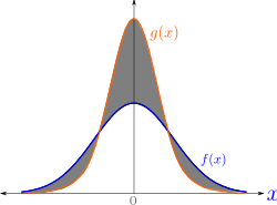
如上图所示,总变差是两条曲线之间绝对面积的一半,也就是上面阴影面积的一半。
设奖励函数有一上界 ,满足
所以也就有
可以推导出
-
若 满足1-利普西茨连续(1-Lipschitz),则 的形式是1-Wasserstein distance:
利普希茨连续是一个比一致连续更强的光滑性条件,限制了函数的斜率,必小于一个实数(该常数依函数而定)。
假设 满足 -Lipschitz 连续,则有
方法(ii)的优点在于它结合了状态空间的几何特性,但代价是需要额外的假设,但这通常在我们的设置中难以验证。另一方面,方法(i)中的假设非常温和且通常在实践中成立。因此,除非我们对MDP有一些先验知识,否则我们应该更倾向于选择方法(i)。我们将上述选项中的假设和不等式总结如下。
参考阅读:Total Variation Distance - wikipedia、Total Variation Distance 总变差 - 知乎、利普希茨连续 - wikipedia、 Distances between probability measures - berkeley、
设 c 是一个常量, 是一个值函数集合,则对所有策略 π 都有
根据 的不同,c 和 也不同。请参考论文的 Appendix A Reminders about integral probability metrics 。
假设我们可以得到一个不确定性量化(uncertainty quantification, UQ),提供了真实误差的一个上界,这个误差估计器用 u 来表示。
如果对所有s,a , 满足
则认为这个误差估计器是可接受的。
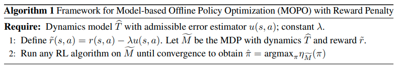
接下来定义 不确定性惩罚的奖励函数(uncertainty-penalized reward):
定义 不确定性惩罚的MDP(uncertainty-penalized MDP):
下式证明了 预测的总奖励函数 将比真实环境中的小,意义是: 是保守的, 可以作为真实环境中 的下界(真值下界)。(由 等式2 和 不等式6 推导而出)
Policy optimization on uncertainty-penalized MDPs
在 Algorithm 1 中优化了 不确定性惩罚的MDP 的策略
Theoretical Guarantees for MOPO
这一部分就是进行对理论性保证进行分析。
先作符号规定:
| Symbol | 含义 |
|---|---|
| 在模型M上的最优策略 | |
| 生成训练数据的策略,行为策略 | |
| 参考上述 Algorithm 1 学得的策略 |
定义 ,对 不确定性量化的期望:
注意, 依赖于 ,但为了简单起见,我们在符号中省略了这种依赖关系。
衡量了在策略 π 的引导下模型的误差:
- 如果,那么 是基于 收集的策略训练的,所以对于 相对来说是准确的,因此 u(s, a) 较小,从而 也很小。
- 另一种情况是,如果策略 π 总是访问数据分布以外的状态,明显 将与 不同。那么 占用量度 所产生的 (s, a) ,将导致误差估计器 u(s, a) 的值也比较大。最终 也很大。
到现在,我们可以推出一个结论:等式10
证明如下:(见论文 Appendix B)
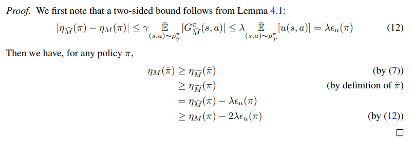
根据上面的 等式 10 有结论:
这表明, 的表现将至少比 要好,因为据前述分析, 很小。
设 ,设 为 在模型误差最大为 δ 的 所有策略中的 最优策略:
学习到的策略 将至少与 模型误差最大为 δ 的 所有策略 一样好,换句话说,当不确定性量化 u(s, a) 足够小时。
将最优策略 带入等式 11,有:
这表明所学习的策略和最优策略之间的 次优性差距(suboptimality gap) 取决于误差 。
越接近数据集,在 上的 u(s, a) 也将更小。动力学模型的不确定性误差越小, 也越小。在极端情况下,u(s, a) = 0,此时有完美的动力学模型和不确定性量化,可以找到最优策略
根据 等式 11 右式,调节 δ 可以平衡return和risk:当 δ 上升时,return 上升,因为 可以从更大的策略范围中学习,增大了探索;然而风险因子 2λδ 也会上升,因此如何选择最优的 δ 是平衡explore与exploit的关键。
我们注意到,δ仅用于分析,并且我们的算法自动实现最佳平衡,因为 等式 11 适用于任何δ。
Practical implementatio
本文的算法基于MBPO。用神经网络构造一个高斯分布作为 动力学模型 ,预测下一状态和奖励:
然后学习一个集成模型(由N个动力学模型 构成,ensemble of N dynamics models),每个模型使用最大似然独立地进行优化。
MOPO与MBPO最重要的区别在于使用了不确定性量化。我们的目标是设计一个 能够捕捉到真实的动力学模型 的 认知不确定性和偶然不确定性 的 不确定性估计器。在理论上已经证明,Bootstrap ensembles能够一致地估计总体均值,并在 model-based RL 中表现良好。与此同时,当模型被正确指定时,高斯概率模型的学习方差在理论上可以重现真实的任意不确定性。
Bootstrap ensembles
贝叶斯神经网络与普通神经网络的区别在于它的权重不再是一个固定的值,而是一个分布,这个分布通常可以是高斯分布,因此一个贝叶斯神经网络是由一个网络+一些权重分布构成的。
我们利用相互独立的数据训练N个贝叶斯神经网络,这些网络的输入为 ,输出为一个分布 。我们把这 N 个网络的输出进行平均,从而得到一个更加鲁棒的输出。
为了得到相互独立的神经网络,需要数据集 {D} 是相互独立的。但是,通常来说我们只需要从 D 中随机采样,得到N个子集就行了。
这个方法在强化学习中基本上还是可行的,它对动力学模型的逼近是比较粗略的,这是因为我们通常不会训练超过10个网络。此外,随机采样也不是必要的,因为SGD和随机初始化已经可以使模型相互独立了。^Model-Based RL: 模型+最优控制器
为了更好的评估不确定性,本文设计使用 学习的 集成模型 的最大标准差 作为 不确定性估计器(uncertainty estimator),使用Frobenius范数的形式:
论文作者选择使用 标准差矩阵范数的最大值 而不是均值,以使策略更加保守和鲁棒。虽然这个估计器缺乏理论保证,但我们发现在实践中它足够准确,能够实现良好的性能。
Frobenius范数是矩阵的一种范数,用于衡量矩阵的大小或矩阵之间的距离,记为 。矩阵A的Frobenius范数定义为矩阵A各项元素的绝对值平方的总和,即
有了这个之后,就要在原始reward上添加penalty。因此,MOPO算法的实际的不确定性惩罚的奖励函数(uncertainty-penalized reward)为:
其中, 是 预测奖励的均值。
惩罚系数 λ 应被视为一个用户选择的超参数。由于我们没有真正的可容许的误差估计器,上述理论中规定的 λ 值在实践中可能不是最优选择;如果我们的启发式函数u(s, a)低估了真实误差,则 λ 应该更大,而如果 u 高估了真实误差,则 λ 应该更小。
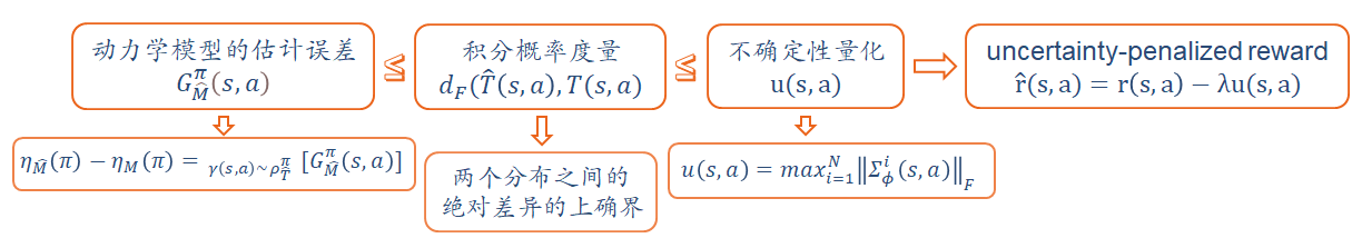
以上部分推导的流程图如下:
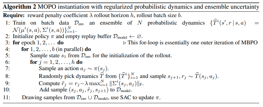
Pseudocode
Experiments/Conclusion/Broader Impact
可参考其他博客。
本文的实验需要验证三个问题:
- 与以前的sota方法相比在offline的benchmark上表现如何
- MOPO是否能够解决泛化到行为分布以外的任务
- MOPO中的各项组件如何影响表现
- D4RL benchmark
- 实验环境:half-cheetah / hopper / walker2d
- 数据集类型:random / medium / mixed / medium-expert
- tasks requiring out-of-distribution generalization
- 两个任务:half-cheetah-jump / ant-angle
- 新环境下的奖励函数需要智能体脱离数据集中的行为策略。
Our work opens up a number of questions and directions for future work. First, an interesting avenue for future research to incorporate the policy regularization ideas of BEAR and BRAC into the reward penalty framework to improve the performance of MOPO on narrow data distributions (such as the “medium” datasets in D4RL). Second, it’s an interesting theoretical question to understand why model-based methods appear to be much better suited to the batch setting than model-free methods. Multiple potential factors include a greater supervision from the states (instead of only the reward), more stable and less noisy supervised gradient updates, or ease of uncertainty estimation. Our work suggests that uncertainty estimation plays an important role, particularly in settings that demand generalization. However, uncertainty estimation does not explain the entire difference nor does it explain why model-free methods cannot also enjoy the benefits of uncertainty estimation. For those domains where learning a model may be very difficult due to complex dynamics, developing better model-free offline RL methods may be desirable or imperative. Hence, it is crucial to conduct future research on investigating how to bring model-free offline RL methods up to the level of the performance of model-based methods, which would require further understanding where the generalization benefits come from.
我们的工作提出了许多未来研究的问题和方向。首先,一个有趣的未来研究方向是将BEAR和BRAC的策略正则化思想纳入奖励惩罚框架,以提高MOPO在狭窄数据分布(如D4RL中的“中等”数据集)上的性能。其次,理解为什么基于模型的方法似乎比基于无模型的方法更适用于批处理设置是一个有趣的理论问题。多个潜在因素包括来自状态的更大监督(而不仅仅是奖励),更稳定且噪声较小的监督梯度更新,或者不确定性估计的简化。我们的研究表明,不确定性估计起着重要作用,特别是在需要泛化的环境中。然而,不确定性估计并不能完全解释整个差异,也不能解释为什么无模型的方法也不能享受不确定性估计的好处。对于那些由于复杂的动力学模型而学习模型可能非常困难的领域,开发更好的无模型离线强化学习方法可能是可取的或势在必行的。因此,未来研究如何将无模型离线强化学习方法提升到基于模型的方法的性能水平至关重要,这需要进一步了解泛化的好处来自哪里。
参考: