MOPO Model-Based Offline Policy Optimization - Simons Institute MOPO讲座

这是Stanford 的 马腾宇 (Tengyu Ma) 在 UC Berkeley 的 Simons Institute 的讲座：MOPO: Model-Based Offline Policy Optimization

Abstract: Offline reinforcement learning (RL) refers to the problem of learning policies entirely from a batch of previously collected data. In this talk, I will discuss MOPO, a model-based offline deep reinforcement learning algorithm. The gist is to modify existing model-based RL methods by introducing a penalty on the reward based on the uncertainty quantification of the learned dynamics. We maximize the penalized return, which is theoretically shown to be a lower bound for the true MDP’s return. MOPO outperforms standard model-based RL methods and existing state-of-the-art model-free offline RL approaches on offline RL benchmarks.

摘要: 离线强化学习（RL）指的是完全基于先前收集的数据批次来学习策略的问题。在本次讲座中，我将讨论MOPO，一种基于模型的离线深度强化学习算法。其要点是通过引入基于学习到的动态的不确定性量化的惩罚，修改现有的基于模型的RL方法。我们最大化惩罚回报，理论上被证明是真实MDP回报的一个下界。MOPO在离线RL基准测试中表现优于标准的基于模型的RL方法和现有最先进的基于无模型的离线RL方法。

Lecturer

Okay, cool, thanks for coming. Thanks for the introduction. This is John, working with Tianku Kevin Yu, Gary Thomas, and Howie Stefano Erman James Zoe. Circuit 11 and Chelsea Finn, I’m Tony Ima from Stanford University. I guess everyone else is also from Santa Fe University, except Sergey who is from Berkeley. So, this is about model-based offline policy optimization.

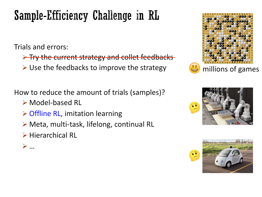
Sample-Efficiency Challenge in RL

I guess, um, let me start with the motivation of studying offline or at least my motivation of studying offline. The bigger picture is that there’s a simple efficiency challenge in applying RL to many real-world applications, as we all know that RL is about trial and error. The technical flow is that you say, “I’m going to try the current strategy and collect feedbacks, and then I’m going to use the feedbacks to improve the strategy.” So, this is a trial-and-error process, and we know how to solve this using this “self-go,” for example, as long as we can try millions of games on a computer. However, in reality, if you use this for robotics or self-driving cars, then potentially you may have the problem that there are not enough samples you can collect from the real environment due to some physical or safety constraints. So, the question is, how do we reduce the amount of trials, the amount of samples we need to implement RL in real applications? One idea is model-based RL, which is considered a promising direction to reduce sample complexity. Another one is offline RL, which I’m going to talk about in a moment. There are also other ways, such as meta, multi-task, lifelong, and continuous RL, which are ways to amortize the cost, and maybe hierarchical, which could also reduce sample complexity. In this talk, I’m going to talk about offline RL, and the approach is model-based. In a nutshell, offline RL is about not having trials and hours to collect feedbacks from the real environment by trying your strategy.

让我们从离线学习的 motivation 开始。大的背景是，在将强化学习应用于现实世界中存在一个明显的效率问题，我们都知道强化学习是通过试错来实现的。技术流程是这样的：“我要尝试当前的策略并收集反馈，然后我要利用这些反馈来改进策略。”所以，这是一个试错的过程，我们知道如何使用“自我对弈”来解决这个问题，例如只要我们可以在计算机上尝试数百万次游戏。

然而，在现实中，如果你将其用于机器人或自动驾驶汽车，那么可能会出现这样的问题，由于一些物理或安全限制，你可能无法从真实环境中收集到足够的样本。所以问题是，我们如何减少在实际应用中实施强化学习所需的试验次数和样本数量？一个想法是基于模型的强化学习，被认为是减少样本复杂性的一个有前途的方向。另一个是离线强化学习，这个我马上就会谈到。还有其他方法，比如元学习、多任务学习、终身学习和连续学习，它们是分摊成本的方法，也许还有分层学习，可以减少样本复杂性。

在这次演讲中，我将讲授一种离线强化学习算法，该算法是 model-based。简而言之，离线强化学习是指不需要试验和几个小时来通过尝试你的策略从真实环境中收集反馈的方法。

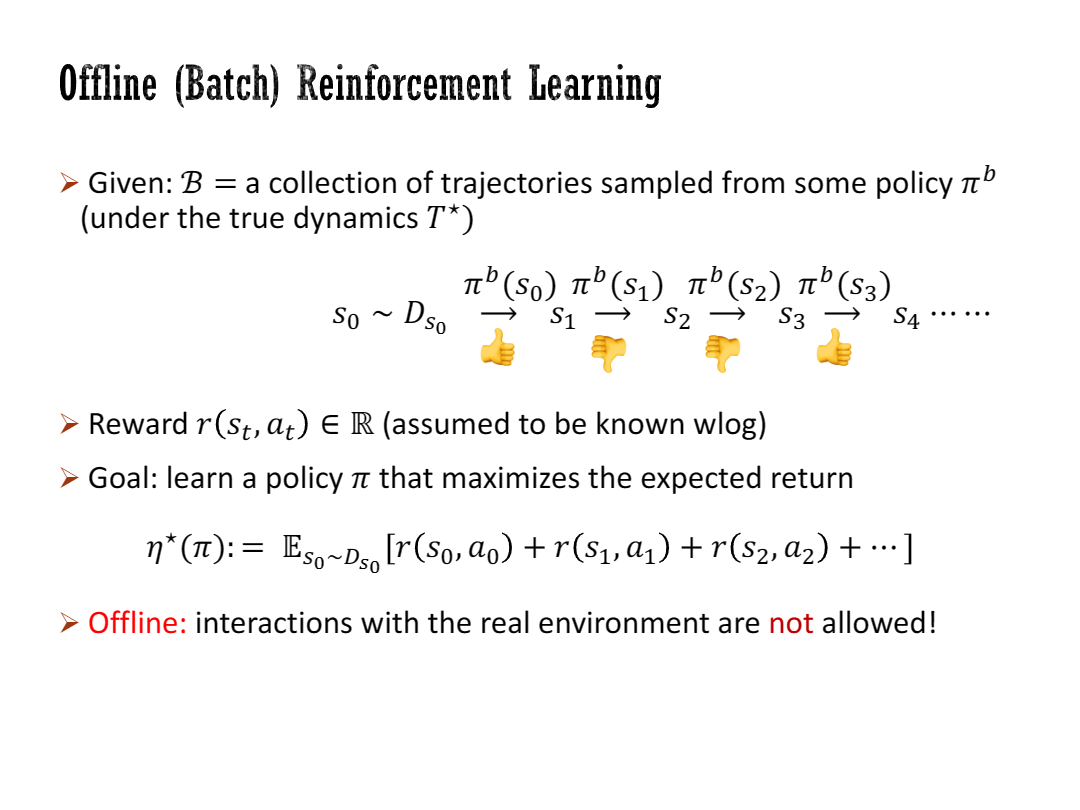
Offine (Batch) Reinforcement Learning

So formally, the definition of offline RL is as follows. Sometimes it’s also called batch reinforcement learning. We are given a batch of data, a collection of trajectories sampled from some policy $\pi_b$, sometimes called the behavior policy, and sometimes it’s actually collected from a mixture of different policies. This collection of trajectories is sampled from the real environment, the true dynamics $T^{\star}$, and we start from $s_0$ and execute this policy $\pi_b$ to get the structures and rewards. Our goal is to learn a policy that maximizes the expected return on the real environment. The expected return is the sum of the return over time, with the expectation over the randomness of the initial states and the randomness of the policy π. Offline really means that we don’t have any additional interactions with the real environment, so after seeing this trajectory of samples, you cannot interact with the real environment.

正式来说，离线强化学习的定义如下。有时也称为批量强化学习。我们被给定一批数据，即 一组从某个策略$\pi_b$（有时称为行为策略）采样得到的轨迹 ，有时实际上是从不同策略的混合中收集的。这些轨迹的采样是从真实环境，真实的动态情况 $T^{\star}$ 中进行的，我们从初始状态$s_0$开始执行策略$\pi_b$，以获得状态和奖励。我们的目标是学习一个策略，使得在真实环境中期望回报最大化。期望回报是随时间的回报之和，其中期望是在初始状态的随机性和策略π的随机性上求取的。离线实际上意味着我们没有与真实环境的任何其他交互，因此在看到这些样本轨迹之后，你不能与真实环境进行交互。

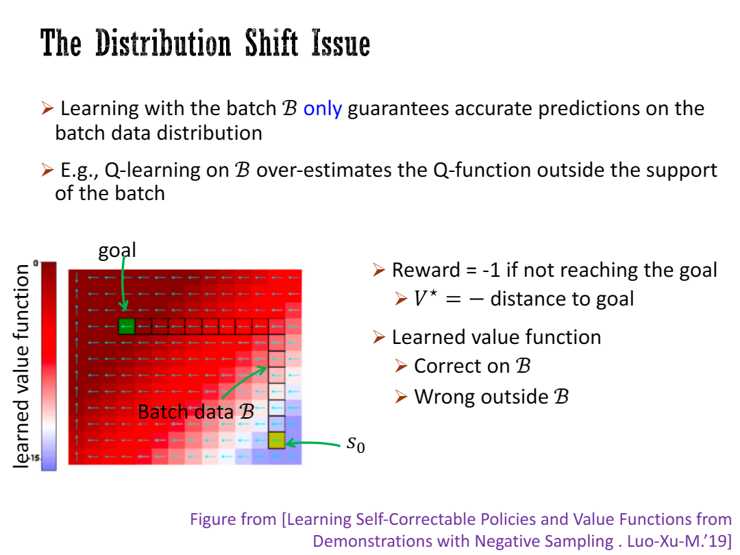
Distributional Domain Shift

It’s well known that there’s a so-called distribution shift issue, for offline reinforcement learning. Roughly speaking, anything you learn from the batch only guarantees accurate predictions on the batch data distribution. The extrapolation to outside the batch data execution is not guaranteed. So, if you execute your policy, you’ll learn some policies that have to go outside the batch distribution, then there’s a domain shift issue. For example, this domain shift could be damaging if you learn your q function on a batch and then it may overestimate the q function outside the support of the batch. Here is a simple experiment. We have a grid world example. There’s an initial state at zero, and a unique goal. You can go left, upward, rightward, and so forth. We have some batch data, which is only a single trajectory from the initial state to the goal. If you learn on the batch data the value function using either kind of Bellman equation or some color approach, then what you see is that the value function learned on the batch is pretty correct on the batch itself, but it wrongly extrapolates outside the batch. The value function actually linearly extrapolates, so the largest value function is obtained on the top-left corner, which is clearly wrong because the large value should be at the goal. This extrapolation outside the batch is wrong and damaging because if you use this value function to induce some policy, even assuming you have the true dynamics, then you’re going to just follow the arrows and go to the top-left corner instead of going to the goal.

众所周知，离线强化学习存在所谓的分布偏移问题。粗浅地说，你从批量数据中学到的任何东西只能保证在批量数据分布上进行准确预测。对于数据集外之外的执行情况，无法保证预测的准确性。因此，如果你执行你的策略，学到的一些策略必须超出数据集数据的分布，那么就会出现领域偏移问题。例如，如果你在数据集的数据上学习了Q函数，然后在数据集外高估了Q函数，这种分布偏移可能会对算法的性能造成损害。

以下是一个简单的实验。我们有一个网格世界的例子。初始状态在零点，还有一个唯一的目标。你可以向左、向上、向右等方向移动。我们有一些批量数据，只是一条从初始状态到目标的轨迹。如果你在批量数据上使用贝尔曼方程或其他方法学习值函数，那么你会发现在数据集内的数据上学到的值函数在批量数据本身上是相当正确的，但在数据集之外却错误地进行了外推。值函数实际上是进行线性外推的，因此最大的值函数在左上角得到，这显然是错误的，因为最大的值应该在目标处。这种对数据集之外的外推是错误和有害的，因为如果你使用这个值函数来引导某个策略，即使假设你在真实的环境中，你也会只是按照箭头的指示去到左上角，而不是去目标处。

A Common Idea: Strong Pessimism/Conservatism

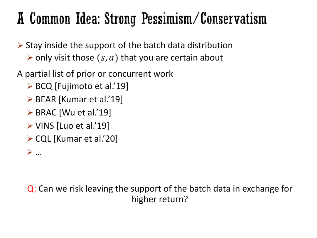
A common idea to deal with the domain shift or distribution shift issue is what I call “strong passive pessimism” or “strong conservatism”. I’m just inviting this word for contrasting with the slightly milder conservatives I’m going to talk about in this talk. So basically, the idea is that you should stay inside the support of the batch data distribution. In other words, you only want to visit those states that you are very certain about. This is kind of the basic idea in many of the prior works. Here, BCQ, BEAR and BRAC are model-based approaches which try to restrict the action to be close to the action that we have seen. Vince and CQL try to penalize either the value function or the Q function outside the batch data distribution.The question we are asking here, one of the motivating points for us to design an algorithm, is whether we can risk leaving the support of the batch data in exchange for a higher return. Sometimes you want to leave the support of the batch data because there’s a better approach to achieve the goal. However, we are less certain about leaving the support; we have to take the risk and balance it for a higher possible return.

处理分布偏移问题的一种常见思路是我所称的“强烈的被动悲观主义”(strong passive pessimism) 或“强烈的保守主义”(strong conservatism)。我只是用这个词来对比一下我在这个演讲中要谈到的稍微温和的保守主义。

基本上，这个想法是你应该保持在数据集分布的支持范围内。换句话说，你只想访问那些你非常确定的状态。

这在许多之前的工作中都是基本思想：BCQ，BEAR和BRAC是基于模型的方法，试图限制动作，以接近我们所见过的动作。VINS和CQL则试图对数据集分布之外的值函数或Q函数进行惩罚。

我们在这里提出的这个问题，是我们设计算法的一个动机之一——就是我们是否可以冒险离开数据集的支持范围，以换取更高的回报。有时你想离开数据集的支持范围，因为有更好的方法来实现目标。然而，我们对离开支持范围的情况不太确定，我们必须冒险并在可能的更高回报中进行平衡。

Simplification: Offline Multi-Arm Bandit

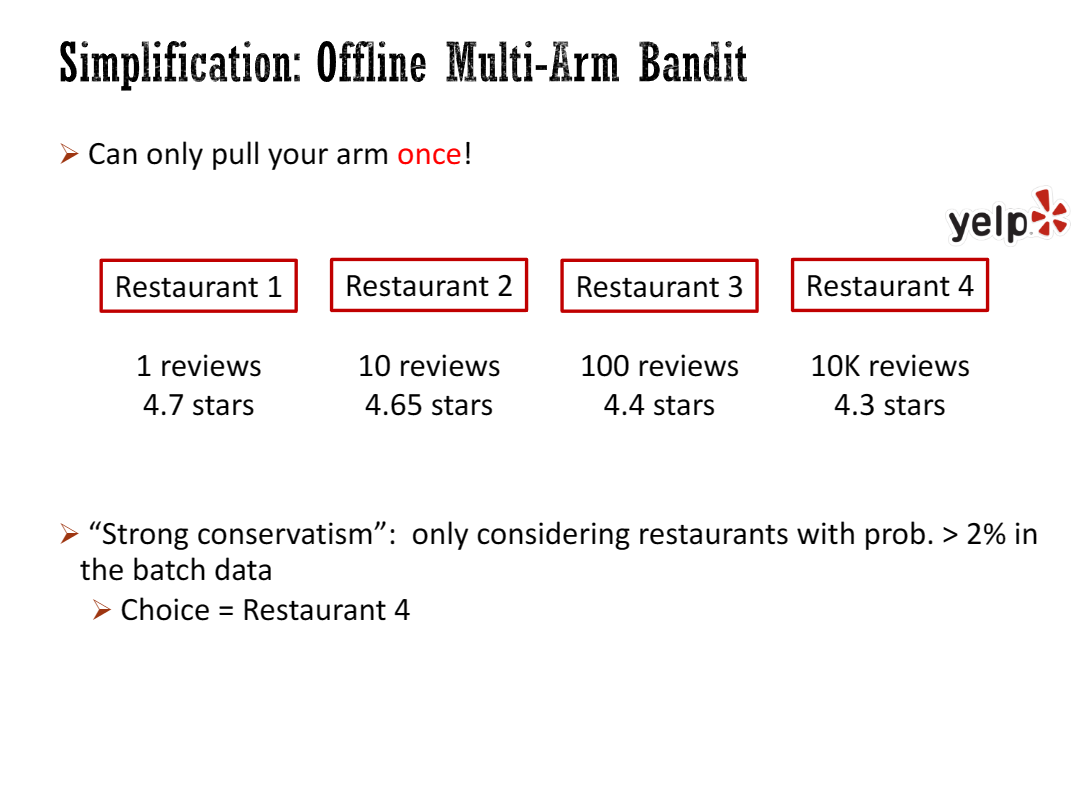
Let me demonstrate the main idea of the talk, which is actually very simple, on a simple toy case: the offline multi-armed bandit problem. This is a dramatic simplification, but it turns out to be almost the same as offline reinforced learning, at least from the perspective of this talk. This is basically my mandate, but you can only pull your arm once. It’s like you are doing the last bet in the casino, and you have to go home after this. You cannot do any trials and errors anymore. I’m not going to use the casino as an example; I’m going to use Yelp. Let’s say there are four restaurants. You have some past reviews for these four restaurants. Let’s assume that the reviews are independent and now you have to choose one restaurant to go to. You want to maximize the taste, maximize the stars of the restaurant. Here, I have been in this kind of situation where for some restaurant you only have one review, and for some other restaurants, you have 10k reviews, and they have different mean stars.

让我在一个简单的案例中展示这个演讲的主要思路，这实际上非常简单：离线 多臂老虎机问题。这是一个极端简化的情况，但从这个演讲的角度来看，它几乎与离线强化学习相同。

这是我给你布置的任务，但你只能拉一次摇杆。就像你在赌场做最后一次赌注，然后你必须回家。你不能再进行任何试验和错误了。

这里，我不打算以赌场为例子，我打算用Yelp(类似大众点评)来说明。假设有四家餐厅，有一些对这四家餐厅的历史评论。假设评论是相互独立的，然后现在你必须选择一家餐厅去。你想最大化你尝到的美味，也就是最大化餐厅的星级评价。

我曾经遇到这种戏剧性的情况，对于某些餐厅，你只有一条评论，而对于其他一些餐厅，你有1万条评论，它们的平均星级不同。

Milder Conservatism: Trading off Return with Risk

If you apply the strong conservatism approach to this multi-armed bandit problem in an offline setting, that means you should consider staying in the support of the batch distribution. Of course, the support is not a well-defined notion in some sense because it’s not robust to any small perturbation. So I’m interpreting the support here as that you need to have enough density in the batch data—this is also what the prior work is trying to use. You need to stay approximately where the density is sufficiently large.

Suppose you only consider restaurants with at least a two percent probability in the batch data. If you make the two percent cutoff, you have to choose restaurant four because that’s the only restaurant with more than two percent of the reviews in the batch data. That means you can only choose restaurant four; only for restaurant four, you have sufficient data to be certain.

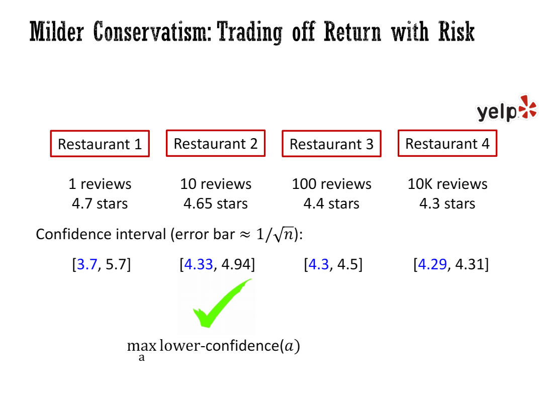
However, what we are going to do is be a little milder, a little less conservative, by considering trading off the risk with the return.

So what we do is we characterize the risk. We compute the confidence interval for each restaurant—upper confidence bound and lower confidence bound. Then we maximize the lower confidence bound of this biased confidence interval. We take the action that maximizes the lower confidence interval and choose restaurant two, which guarantees a trade-off between the risk and return.

This is the main idea of this paper. Here is a super-trivial multi-armed bandit, and the only thing we have to do is to extend this to reinforcement learning.

如果你将强保守主义方法应用于离线环境中的多臂老虎机问题，这意味着你应该考虑停留在数据集的支持范围内。当然，在某种意义上，这个支持范围并不是一个明确定义的概念，因为它对任何小的扰动都不具有鲁棒性。所以在这里，我将支持范围解释为你需要在批量数据中有足够的密度（占比） - 这也是之前的工作试图使用的方法。你需要停留在密度足够大的地方。

假设你只考虑在批量数据中至少有2%概率的餐厅。如果你设定了2%的截断值，那么你只能选择餐厅四，因为只有餐厅四的评论超过了批量数据中2%的比例。这意味着你只能选择餐厅四；只有对于餐厅四，你才有足够的数据来确信它的评论。

然而，我们要做的就是稍微温和一些，稍微不那么保守，来权衡风险和回报。

所以我们要做的是对风险进行量化。我们计算每个餐厅的置信区间 - 上置信界和下置信界。然后我们最大化这个有偏置的置信区间的下置信界。我们选择最大化下置信界的行动，并选择餐厅二，这就保证了风险和回报之间的权衡。

这就是这篇论文的主要思想。这是一个非常简单的多臂老虎机问题，我们唯一需要做的就是将其扩展到强化学习中。

Back to offline reinforced learning

So the first step is that we build a certain qualification of the return, so we say we want to make sure eta star pi, this is the true return on the true dynamics to be in some interval. You can hide pi plus minus e of pi.

And then after you get this certain quantification, you say, “I’m going to maximize the lower confidence bound.” It had pi minus e of pi, and then um then that’s the two steps. So basically, this is what this talk is about, and I’m going to describe a little bit how do I do step one, and step two is pretty simple, basically, you just apply some optimization algorithm optimizing over the policy.

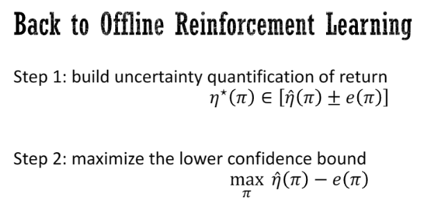
所以第一步是我们建立一个回归的一定条件，我们定义不确定性量度(UQ) $\eta^{\star}(\pi)$，这是在某个区间内的策略 π 在真实环境下期望回报 $\hat{\eta}$ 的一个上下界。你可以隐藏 $\hat{\eta}(\pi)\pm e(\pi)$。

然后在你得到这个确定的量后，我们可以最大化置信下限。它就是$\hat{\eta}(\pi)-e(\pi)$。这是两个步骤。所以基本上，这就是这次演讲的内容，我将稍微描述一下我如何进行第一步，第二步非常简单，基本上，你只需应用一些优化算法来优化策略。

Step 1: Uncertainty Quantification (UQ) For the Return

So how do we build a certain classification for the return? We are taking a model-based approach, meaning that we are starting from the uncertainty quantificationfor learning dynamics, and then we translate that uncertain quantification for the dynamics to an uncertain classification for the return.

So we don’t know how to do the answer signification for the learned dynamics in a principled way. This is a very difficult way different question, so any answer modification with a nonlinear model is difficult, but we assume we have a building block or module or kind of oracle to have an identification for the learned dynamics, and then we turn that into a certain quantification for the return of the policy.

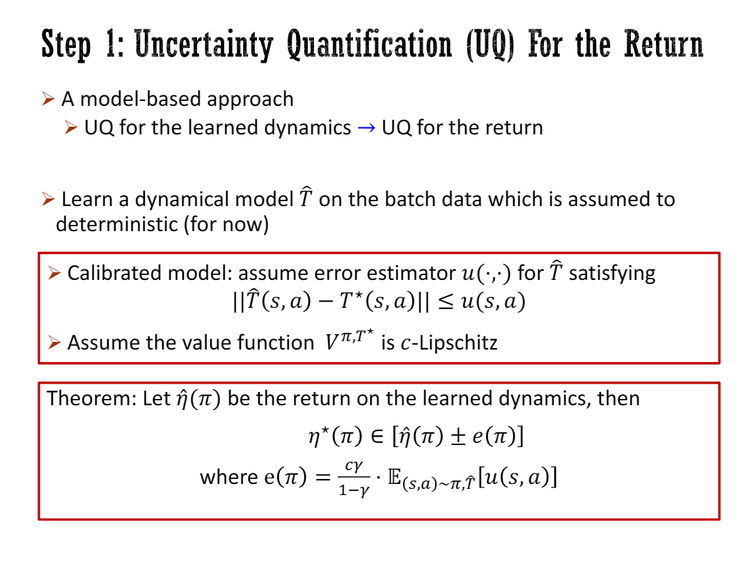
So how do we do that? We learn a dynamical model that on the batch data, which is assumed to be deterministic for the moment. I’m going to extend it to stochastic case as well. So, and we also assume that the learning, so because learning dynamical model is surprised, so we assume that the surprise learning algorithm also comes with a calibrated guarantee.

Calibration guarantee, so assume that there exists an arrow estimator. We can obtain an arrow estimator u for the dynamics that satisfying that the arrow estimator u is admissible.In the sense that it’s indeed an upper bound for the real error. So that hat minus t star, the norm of that hat and c star. So this is our assumption on the calibration of the model.

And then we also assume that the value function v pi t star is the ellipsis. I’m going to expand on this a little bit on the next slide, but basically, you have to assume something about your value function. Oh, because you know you have to assume something about the reward function, right? If the reward can be plus minus infinity, then there’s no chance that you can do anything offline because the reward at some other state you haven’t seen could be just a plus infinity or negative infinity.

And then with these assumptions, we can prove that you have some external quantification. So this is a confidence bound for eta star. So eta star is in either hat pi plus minus e of pi, and e of pi is equals to this quantity. It’s a scalar c gamma c gamma over one minus gamma times the expectation of usa, the expectation of the arrow estimator over on the trajectories sampled from the policy pi and the learn dynamics that hat.

So this error estimator, so this e pi is something we can compute ourselves if we have the error estimator u and also the policy pi and that hat. So I guess I see a question, is the right thing to do to answer the question right now? Go ahead and answer it, that’s fine. Sure, okay.

Yeah, so the question is, is it maximizing the lower bound confidence bound kind of exploration versus exploitation dilemma while being conservative with the lower bound only? So I guess here, you know, this is a very good question. So why we are optimizing the lower confidence bound. So it sounds like this is still very conservative. I agree, this is still very conservative. We are just treating off with the return a little bit, and part of the reason we do this is that this guarantees that we can have a lower bound for the real return. But potentially there could be better ways to do it. I will discuss this probably more at the end in the open questions.

This is basically the how the reason we do this is that this guarantees that we can have a lower bound for the real return. Potentially, there could be better ways to do it. I will discuss this more at the end, in the open questions.

那么我们如何为回报建立一种特定的分类？我们采用基于模型的方法，意味着我们从学习动态的不确定性量度(UQ)开始，然后将该不确定性量度转化为对回报的不确定性量度。

因此，我们不知道如何以一种有原则的方式对所学的动力学模型进行显著性检验。这是一个非常困难的问题，所以任何使用非线性模型进行的答案修改都很困难，但我们假设我们有一个构建块、模块或某种预言机，可以对学习到的动力学模型进行识别，然后将其转化为策略回报的一定量化。

那么我们该如何做到呢？我们在批量数据上学习一个动态模型，暂时假设该数据是确定性的。我也将把它扩展到随机情况。因为学习动力学模型是启发式，所以我们假设启发式的学习算法也具有校准保证。

校准保证意味着假设存在一个误差估计器。我们可以得到一个对于动态模型的误差估计器u(:,:)，如果满足 $||\hat{T}(s,a)-T^{\star}(s,a)||\leq u(s,a)$ 则认为u是一个可接受的误差估计器。即它提供了真实误差的一个上界。（证明请见其他博客和论文）所以这是我们对模型校准性的假设。

然后我们还假设值函数$V^{\pi,T^{\star}}$是省略的。我将在下一张幻灯片上详细展开，但基本上，您必须对您的值函数做出一些假设。因为您知道您必须对奖励函数做出一些假设，对吧？如果奖励可以是正无穷或负无穷，那么您无法在离线状态下做任何事情，因为您尚未见过的某个其他状态的奖励可能是正无穷或负无穷。

在这些假设的基础上，我们可以证明您有一些外部量化。这是 $\eta^{\star}(\pi)$的置信区间。所以 $\eta^{\star}(\pi)$ 在区间$\hat{\eta}(\pi)\pm e(\pi)$内，其中$e(\pi)$等于这个量。它是一个标量，$\frac{c\gamma}{1-\gamma}\cdot\mathbb{E}_{(s,a)\sim\pi,}[u(s,a)]$。

这个误差估计器$e(\pi)$是我们自己可以计算的，如果我们有误差估计器u、策略pi和动力学模型$\hat{T}$的话。所以我猜我可以回答这个问题，现在回答也可以，没问题。

所以，问题是，在保守地处理下界的情况下，是否最大化下界置信区间会导致探索与开发的困境？我想这是一个非常好的问题。为什么我们要优化下界置信区间呢？听起来这仍然非常保守。我同意，这确实非常保守。我们只是稍微权衡了一下回报，我们这样做的部分原因是这样可以保证我们对真实回报有一个下界。但可能还有更好的方法来处理这个问题。我可能会在最后的开放问题中进一步讨论这个问题。

好的，基本上这就是我们这样做的原因，这可以保证我们对真实回报有一个下界。可能还有更好的方法来处理这个问题。我将在最后的开放问题中进一步讨论这个问题。

Unified Approach for Stochastic Dynamics

We use the ISO and configuration for the dynamics and turn it into a simplification for the right term. You can also have a unified approach for stochastic dynamics.

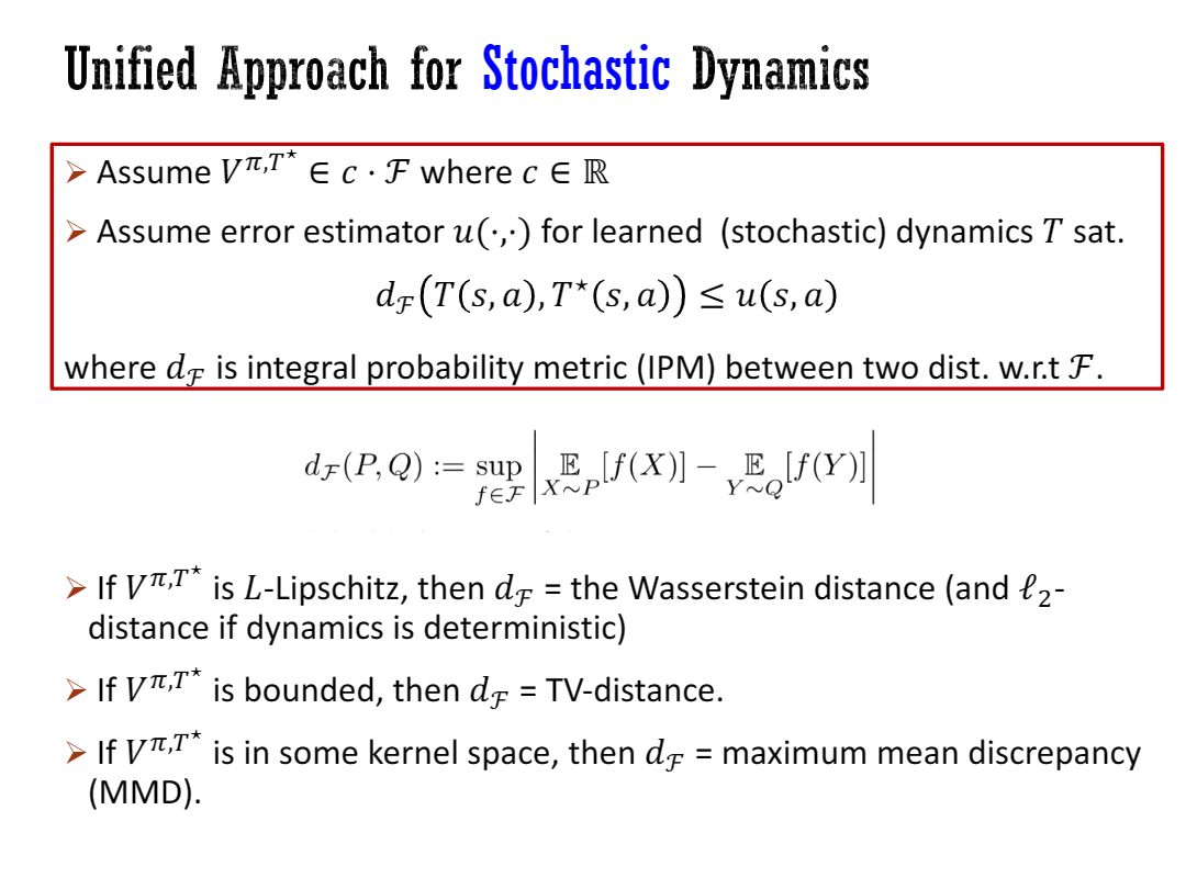
Here, what we do is that this page is a little bit abstract, but bear with me for a moment. We assume that the value function belongs to some C times a scalar times the family of functions F. We assume some error estimator in a slightly different form. We assume that, because this is um, stochastic dynamics, then T of S, A, and T-star of S, A are random variables or distributions. So then we measure the quality of the dynamics by estimating the distance between T-star of S, A and here the distance is the integral probability metric (IPM) between the two distributions with respect to F. We want the average meter to be an upper bound of that.

To remind you, the IPM is a way to measure the distance between two distributions via the test function F belonging to the family F. You look at the expectation of F under the two distributions, take the differences, and then take the sup over all the test functions. This allows us to unify a few different cases. For example, if you assume V-pi-T-star is L-Lipschitz, then the distance is the Wasserstein distance. If the dynamics are deterministic, then the distance is just the L2 distance. If V-pi-T-star is bounded, then the distance is the total variation distance. If T-star is some kind of kernel space, then df could be the maximum mean discrepancy distance.

==暂时还没看懂==

上图中 w.r.t 指 with respect to，关于。

我们使用ISO和动力学模型配置，并将其转化为对右侧项的简化。您还可以对随机动力学模型采用统一的方法。

在这里，我们做的是有点抽象的，但请稍等片刻。我们假设值函数 V 属于 某个c(标量) × 函数族 $\mathcal{F}$ （设 $\mathcal{F}$ 为 从 $\mathcal{S}$ 映射到 $\mathbb{R}$ 的一个函数集合，其中包含了 $V_{M}^{\pi}$ ）。我们以稍微不同的形式假设了一些误差估计器。我们假设，因为这是随机的动力学模型，所以$T(s,a)$和$T^{\star}(s,a)$是随机变量或分布。因此，我们通过估计$T(s,a)$和$T^{\star}(s,a)$的距离，也就是 积分概率度量(IPM) 来衡量动力学模型的质量。我们希望平均量是其上界。

So then we measure the quality of the dynamics by estimating the distance between T-star of S, A and here the distance is the integral probability metric (IPM) between the two distributions with respect to F.

应用两种距离公式进行对比分析：

提醒一下，IPM是通过测试函数F来衡量两个分布之间的距离的一种方法，其中测试函数F属于函数族F。您观察两个分布下的F的期望，取差值，然后对所有测试函数取上确界。这使我们能够统一几种不同的情况。

例如，如果假设$V^{\pi,T^{\star}}$满足L-Lipschitz，则距离是Wasserstein距离。如果动力学是确定性的，则距离只是L2距离。

如果$V^{\pi,T^{\star}}$有界，则距离是总变差距离(total variation distance, TV-distance)。

如果$V^{\pi,T^{\star}}$是某种内核空间，则df可以是最大均值差异距离。

With this, we can prove almost the same result, but just with a more general assumption. So, it’s basically the same guarantee. We know that E of pi of the same form is our estimator for the true return.

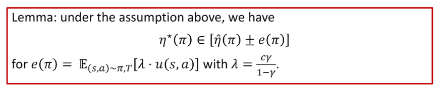
通过这种方法，我们可以证明几乎相同的结果，只是基于一个更一般的假设。因此，基本上是相同的保证。我们知道$e(\pi)$具有相同的形式，它是我们对真实情况下return的估计器。

Proof Sketch

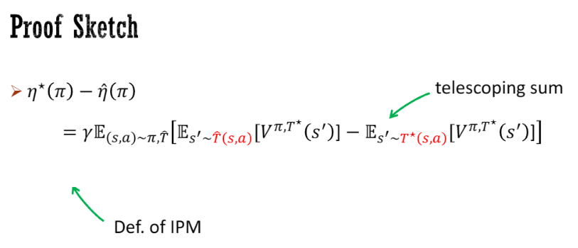
I’m going to escape the proof sketch. I will just flash it because I have limited time. The proof sketch is simple. It has been done in prior work. Basically, you’re trying to build the upper bound for eta star pi minus eta hat pi in the height path, which is the return on the virtual environment. It has star pi, which is the return on the real environment. The first step is to do some kind of telescoping sum (detailed explanation skipped). The test concept was instant expectation, a way to measure the differences between that and t star under the test function of v pi. You then use the IPM definition and change it to IPM, knowing that IPM is less than the u(s,a).

$\eta^{\star}(\pi)$ 在区间$\hat{\eta}(\pi)$

==暂时还没看懂==

我打算略过证明草图，我只会快速浏览一下，因为时间有限。这个证明草图很简单。之前的工作已经完成了。基本上，你正在尝试建立以$\eta^{\star}(\pi)$ 减去 $\hat{\eta}(\pi)$ 在高度路径上的上界，这是虚拟环境的回报。$\eta^{\star}(\pi)$是真实环境的回报。第一步是进行一些类似于望远镜的求和（跳过了详细解释）。测试概念是即时期望，一种用于衡量与测试函数vπ下的t星之间差异的方法。然后，你使用IPM定义并将其转换为IPM，知道IPM小于u(s,a)。

MOPO: Model-based Policy Opt. with Reward Penalty

With this configuration, we can do a second step, which is the model voice-based policy optimization with the reward penalty. In the second set, we are trying to optimize pi. The lower bound e to pi minus e of pi can be written as the expectation of r of x a minus lambda of u of s. Since what’s under the expectation is the same, you can merge them together into a single expectation. You realize that this is basically optimizing the policy for penalized MDP and tilde, which is defined to have the same learned dynamics t hat and the penalized reward are tilde, which is penalized by lambda times the answer implication of the dynamics. Some off-the-shelf algorithms can be used to optimize it. How do we implement the iso multiplication for dynamics? I’ve thought about this for a while, and it turns out there aren’t many good ways to do iso convocation, especially under out-of-domain shift for even surprise learning. So what we do is just a heuristic. We use the ensemble to do a heuristic for UFX. We take a sample of models and look at the differences between their outputs.

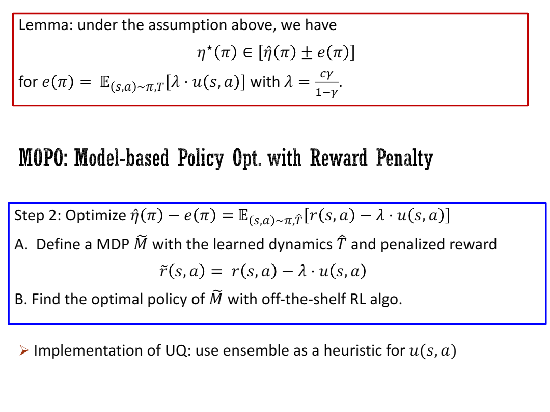
有了这个配置，我们可以进行第二步，即基于模型的声音策略优化与奖励惩罚。在第二个集合中，我们试图优化π。下界e到π减去e的π可以写成r的x a减去λ的u的s的期望。由于期望下的内容相同，可以将它们合并为一个单一的期望。你会意识到，这基本上是为受惩罚的MDP和tilde优化策略，tilde被定义为具有相同学习动态t hat和受惩罚奖励的tilde，其受到动态的λ倍数的惩罚。可以使用一些现成的算法来优化它。我们如何实现动态的iso乘法？我思考了一段时间，结果发现没有太多好的方法来进行iso卷积，尤其是在域外转移和意外学习的情况下。所以我们只是使用一种启发式方法。我们使用集合来对UFX进行启发式处理。我们取样多个模型并观察它们输出之间的差异。

==暂时还没看懂==

Characterizing the Tradeoff between the Gain and Risk of Leaving Batch Data Support

Running a bit late, so I’ll skip the slice. I start the motivated talk by talking about the trade-off between the gains and the risk of leaving batch support. We can also characterize that a little bit. Um, this is just a super simple extension of the theorem. So basically, you can characterize what the property of the policy is. It’s kind of like doing some kind of trade-off between taking the risk of our maximizing the return. It just takes, uh, it’s trading off between having smaller risk and maximizing the return. Here, the policy is larger than Ether star pi minus 2 lambda times absolute pi. Absolute pi is a way to measure the risk and basically you are treating all these two terms.

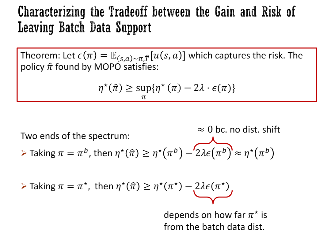
在谈论离开批量支持的收益和风险之间的权衡时，可以进行激励性的讨论。我们还可以对此进行一些特征描述。这其实只是定理的一个非常简单的扩展。基本上，你可以描述策略的特性。就像在承担风险和最大化回报之间进行某种权衡一样。这只是在小风险和最大化回报之间进行权衡。

==暂时还没看懂==

Evaluation on D4RL dataset

We did a bunch of evaluation either. So this paper is, you know, even though there’s some theory here, mostly it is about empirical results. So we did an evaluation on the default IO dataset, which is a recently collected, you know, benchmark dataset for offline reinforcement learning. And then we see that our results are better than some of the best methods on batch-fixed environments.

So here, the kind of environments we’re doing pretty well are those kind of so-called mixed or random environment, meaning that here the best data are from a mix of policy or from random policy. So, we suspect that the reason is that we are doing well when the batch data are somehow kind of like diverse. So this allows us to have a good answering classification for dynamics. The dynamics can extrapolate outside the support of the data. However, if the batch data is not diverse enough, like in a medium which means that you only have a single policy in the batch that generates the batch data, and then, the batch data is very kind of like a low dimensional, and the extrapolation of the dynamics is not good. So that’s why our method is not as competitive as in other cases.

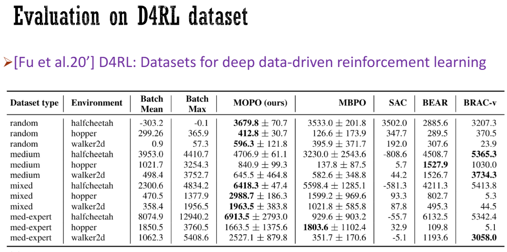
我们进行了大量的评估工作。所以这篇论文，虽然其中有一些理论，但主要是关于实证结果的。因此，我们对最近收集的默认IO数据集进行了评估，这是一个离线强化学习的基准数据集。然后我们发现，我们的结果比一些最好的批处理固定环境方法要好。

在这里，我们表现良好的环境是那些所谓的混合或随机环境，意味着最好的数据来自策略的混合或来自随机策略。因此，我们怀疑原因是当批处理数据在某种程度上具有多样性时，我们在动态分类方面表现良好。动态分类可以在数据的支持范围之外进行外推。然而，如果批处理数据的多样性不够，比如在中等程度的情况下，意味着批处理中只有一个策略生成批处理数据，并且批处理数据的维度非常低，动态外推效果就不好。这就是为什么我们的方法在其他情况下不如竞争对手的原因。

Out-of-distribution Offline RL Tasks

So, we also evaluated our method on the so-called auto-distribution offline RL tasks that we designed. This was to test whether our method performs well in situations where the agent has to take the risk of leaving the support of the batch data to achieve higher rewards. We designed tasks where the batch data and the task itself differ. For example, one of the tasks is called “ant-angle” where the batch data only runs forward on the right-hand side, but the task requires the agent to move in a direction with a 30-degree angle. To solve this task effectively, you have to deviate from the batch data to some extent. Another example is the “cheetah-jump” task, where the batch data shows the cheetah running forward, but the task requires the cheetah to jump slightly. This also requires leaving the batch data distribution.

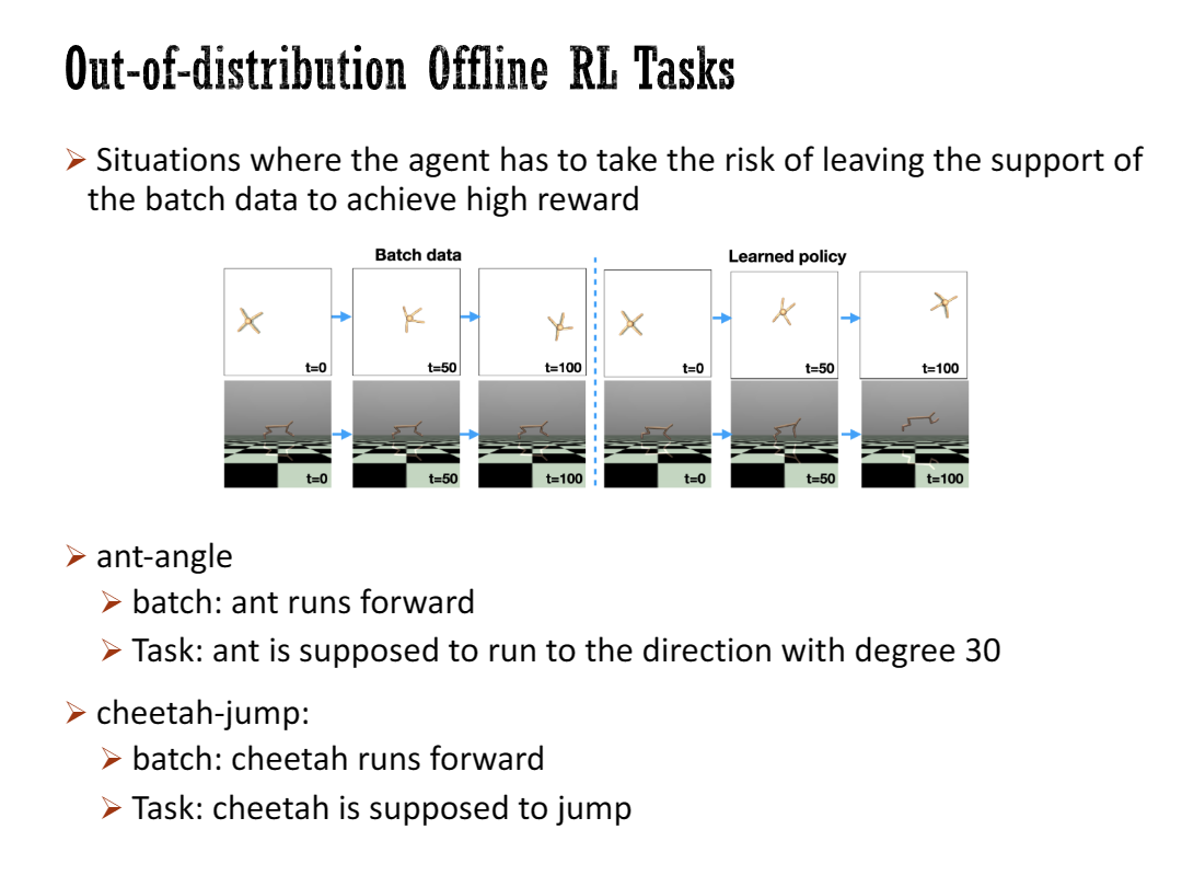
此外，我们还对我们设计的所谓的自动分布离线强化学习任务进行了评估。这是为了测试我们的方法在代理需要冒险离开批处理数据支持范围以获得更高奖励的情况下是否表现良好。我们设计了一些批处理数据与任务本身不同的任务。例如，其中一个任务被称为“ant-angle”，批处理数据只朝右前方移动，但任务要求代理以30度角的方向移动。要有效解决这个任务，你必须在一定程度上偏离批处理数据。另一个例子是“cheetah-jump”任务，批处理数据显示猎豹向前奔跑，但任务要求猎豹稍微跳跃。这也需要离开批处理数据分布。

We can observe that our advantage over prior work is, in some sense, amplified, partly because prior work tends to stay within the batch data distribution.

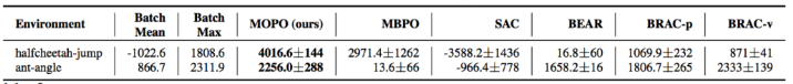
我们可以观察到，与之前的工作相比，我们的优势在某种程度上被放大，部分原因是之前的工作倾向于保持在批处理数据分布内部。

Summary

Okay, so um um just uh the summary so uh this talk is about offline model-based RL. The approach is that we have a reward count from the uncertain quantification of the dynamics, and we just optimize the penalized virtual environment. So, some open questions:

1. One of the obvious open questions is that how do we do tighter and significant um so we have a way to do isolation which is obviously not very tight for many cases.

2. How do we have tighter isolating conditions?

3. Another question is related to some of the questions asked in a talk, so uh how can we be less conservative than optimizing the lower confidence bond? Often the lower confidence bond allows us to show that the thing we are optimizing is a lower bound for the real return, and that gives us some property. However, potentially there’s a way to be less conservative uh uh than doing this uh.

I’d like to spend just one minute to have some advertisements for some of my other iowa work um uh in deep enforcement learning which I spend a lot of time uh these days thinking about some of these questions. One of the work is uh we are studying the differences between model-based RL and model-free RL in terms of expressivity. We show that in many certain cases the Q function can be much more complex to express than the model itself, which suggests that model-based RL probably has some advantage over model-free RL in these kinds of cases. We are also trying to address the distribution shift in math reinforcement by using model-based ideas as well. So i guess this is all i want to say.

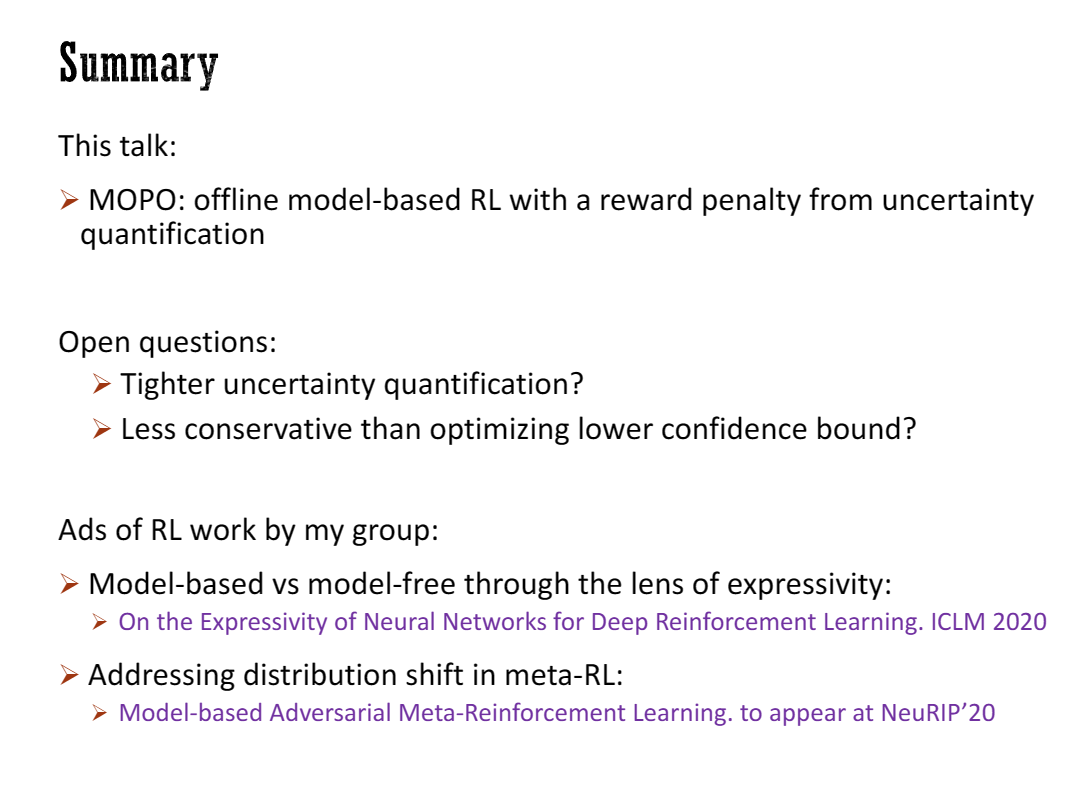
好的，所以这个演讲主要讲述离线模型基于强化学习的内容。方法是通过对动态不确定性进行奖励计数，然后优化受惩罚的虚拟环境。所以，有一些开放性问题：

1. 首先一个明显的问题是，我们如何更紧密和显著地进行隔离，因为目前的隔离方法在许多情况下显然不够紧密。
2. 我们如何获得更紧密的隔离条件？
3. 另一个问题与演讲中提出的一些问题有关，我们如何在优化下限置信区间时更加谨慎？通常，下限置信区间可以证明我们优化的内容是真实回报的下界，这给了我们一些性质。然而，可能有一种方法可以比这种方法更加谨慎。

我想花一分钟为我在深度强化学习方面的其他工作做一些广告，这些天我花了很多时间思考这些问题。我们正在研究基于模型的强化学习和基于模型的强化学习在表达能力方面的差异。我们证明在许多情况下，Q函数的表达复杂度要高于模型本身，这表明在这些情况下，基于模型的强化学习可能具有一些优势。我们还在尝试使用基于模型的思想来解决数学强化学习中的分布偏移问题。所以我想这就是我想说的全部。

Discussion

I was just wondering about this result that relates the model estimation error to the policy value error. So, is this not the simulation? Lambda, this is just a simplification. Oh, I’m not sure whether that’s a common word, but you know. But this is just a simulation. We do a little bit on top of it by doing the one system IPM thing, but you know. But it’s just a simulation, yes, right? But when you, for example, when you try to come up with confidence intervals in terms of what such time distance can you actually like do this for any reasonable class of models or you’re just using it as an abstract example? Um, so if you, I’m just using that as an example, but um, sorry, can you say the last question? Yeah, so like can you derive meaningful bounds on the Wassenstein distance that would lead to like a reasonable algorithm? Um, you know, so um, the Wassenstein distance, so so we are, so after we got the Wassenstein distance, we assume that you have an arrow estimator for the Wassenstein distance, and then there’s nothing like everything is folded in the assumption in some sense. So basically, so there’s a lot of wishful thinking in there. So, uh, I guess TV distance is even less, it’s even more eligible thinking, right? So right, I don’t think in reality you can get a model that can be accurate in TV distance. That sounds like very hard to achieve. So that’s just a full demonstration. Yeah, the disclaimer is basically just a simulation, that’s it. All right, thanks very much.

我只是在想关于这个将模型估计误差与策略值误差相关的结果。所以，这不是模拟吗？Lambda，这只是一个简化。哦，我不确定这是否是一个常用词，但你懂的。但这只是一个模拟。我们通过进行一个系统IPM的操作稍微改进了一下，但你懂的。但这只是一个模拟，对吗？但是，例如，当你尝试根据某个合理的模型类来提出置信区间时，你是否可以为这种时间距离推导出任何有意义的界限，还是只是将其用作一个抽象的例子？嗯，所以如果你，我只是用那个作为一个例子，但是，抱歉，你能再说一遍最后一个问题吗？是的，就像你能够推导出对Wassenstein距离的有意义的界限，从而导致一个合理的算法吗？嗯，你知道，Wassenstein距离，所以我们在得到Wassenstein距离之后，我们假设你对Wassenstein距离有一个箭头估计器，然后在某种意义上，所有东西都包含在这个假设中。所以基本上，这里有很多一厢情愿的想法。所以，我猜TV距离甚至更不可靠，对吗？所以，我认为在现实中很难得到一个在TV距离上准确的模型。那听起来很难实现。所以这只是一个完全的演示。是的，免责声明基本上只是一个模拟，就是这样。

Well, this is not really a question, but I thought that one of the open problems is tighter uncertainty quantification. I just wanted to point out that, uh, there are some talks on Friday that will talk about uncertainty quantification, so if people are interested, that would be something interesting to look at.

嗯，这不算是一个问题，但我认为一个未解决的问题之一是更紧密的不确定性量化。我只是想指出，周五有一些关于不确定性量化的讲座，如果有兴趣的人，可以去看看，可能会有一些有趣的东西。

So it seems like uncertainty quantification, you know, is certainly an important part of what you’re doing, and I was just wondering what your experience was with using ensembles because it seems like, you know, what ensembles are really measuring is sort of the variance in your optimizer. You know, so you can imagine the worst case, you just have an optimizer that completely ignores the data, outputs exactly the same thing every time, you say, you know, great zero epistemic uncertainty. So, uh, how much did you run into that in practice?

所以看起来不确定性量化是你所做工作的一个重要组成部分，我只是想知道你使用集成模型的经验如何，因为看起来集成模型实际上衡量的是你的优化器中的方差。你可以想象最糟糕的情况，你只有一个完全忽略数据的优化器，每次输出完全相同的结果，你会说，太好了，没有认知不确定性。那么，你在实践中遇到这个问题有多少？

So, I think we look at the error, the correlation between the ensemble IRA estimator was the real error. Surprisingly, the correlation is pretty well. So, I think the harder part is, what if you optimize your policy based on that harassment, right? So, if you just take some random policy or take some kind of fixed policy and you look at this iso qualification by the ensembles, I think my experience says that it seems that it’s generally pretty okay. But, however, the tricky part is that if you do some optimization, then you may overfit to the ensemble you have. So, here we are pretty much pessimistic. We are taking the one-step error using our sample and then we take the sum of the errors. That’s what the telescoping or the simulation level is doing. So, that seems to reduce this issue a little bit. So, it’s very hard to kind of overfit code overlay to the ensemble because you are taking the error for every stat and then you take the sum. I’m not sure whether that answers the question, but generally, I don’t really know. Like, for us, it seems to be okay. And also, we have slightly different ways to do that certification. In the paper, we have two ways. One way is that we can learn a stochastic model actually, and you take the maximum of the variance across the five stochastic models like you learned. And another way is you look at differences between the disagreements between the ensembles, and both subnets work pretty fun. One method works a little better than the other. But yeah, but generally, I don’t have much more to say than this. It’s pretty empirical. We just try, try, try these things. Yeah, yeah, thanks.

所以，我认为我们应该看看误差，集成IRA估计器之间的关联就是真正的误差。令人惊讶的是，这种关联相当好。所以，我认为更困难的部分是，如果你基于那种扰动来优化你的策略，对吧？所以，如果你只是采取一些随机策略或者采取某种固定策略，并且你通过集成来查看这种等式合格性，我认为我的经验表明这似乎通常还不错。但是，然而，棘手的部分是，如果你进行一些优化，那么你可能会过度拟合你所拥有的集成。所以，在这里我们非常悲观。我们使用样本来计算一步误差，然后将误差求和。这就是迭代或者模拟级别所做的。所以，这似乎在一定程度上减少了这个问题。所以，很难对集成进行过度拟合，因为你对每个统计量都进行了误差计算，然后将其求和。我不确定这是否回答了问题，但总的来说，我真的不知道。对我们来说，似乎还可以。而且，我们有稍微不同的方法来进行认证。在论文中，我们有两种方法。一种方法是实际上可以学习一个随机模型，然后取得你学到的五个随机模型之间方差的最大值。另一种方法是查看集成之间的差异，两种子网都很有趣。其中一种方法比另一种方法稍微好一点。但是，总的来说，我没有更多要说的了。这是非常经验性的。我们只是尝试了这些东西。是的，是的，谢谢。

I want to ask a slightly leading question, but maybe this will be interesting to discuss. So, I’ll just say one last question from you and then we’ll switch to Emma. Thank you. Um, so, you said that you need to do uncertainty quantification, but I wonder if maybe the problem is actually a little bit easier than that because all that’s really needed by the algorithm is some notion that this is like a bad place to be. And I wonder if that’s actually easier than uncertainty quantification for as an example. So, there’s a question in the Q&A about upper bounds versus lower bounds and exploration exploitation that got me thinking about this. If you do count-based exploration, that is kind of estimating uncertainty in a state, but estimating account is easier than estimating epistemic uncertainty on a model. So, I wonder what your opinion is on whether there’s basically an easier way that doesn’t require the full posterior. I see.

我想问一个稍微引导性的问题，但也许这会有趣讨论一下。所以，我只会从你这里问最后一个问题，然后我们会转到Emma。谢谢。嗯，你说过你需要进行不确定性量化，但我想知道也许问题实际上比那更容易一些，因为算法真正需要的只是一种这是一个糟糕的地方的概念。我想知道是否这实际上比例如不确定性量化更容易。所以，在问答环节中有一个关于上界与下界以及探索与开发的问题让我想到了这个。如果你进行基于计数的探索，那就是在估计状态的不确定性，但是估计计数要比估计模型的认知不确定性容易。所以，我想知道你对于是否存在一种不需要完整后验概率的更容易的方式的观点是什么。我明白了。

So, yeah, I guess so. I guess I don’t quite know. So, this is, you know, this is very… This is kind of like what I’m asking, I guess. You know, I’m not sure exactly if I’m interpreting the question in the right way, but this is kind of like what I was thinking about. Less being less conservative. But, on the other hand, I guess at least the thinking from a theoretical perspective, you know, if you’re less conservative, then sometimes, I ask myself, like, do I have any guarantees? So, finding the right middle ground seems to be the hardest part. And also, I guess another… Maybe not answering exactly a question, but one question is, how do we extrapolate to the unseen states? So, if you want to do well, do you have to extrapolate as much as possible to an unseen state? And which mechanism are you relying on? So, are you relying on the model to extrapolate or are you relying on the Q function to extrapolate? Or are you relying on something more advanced to extrapolate? That’s something I assume is also an interesting open question.

嗯，是的，我想我不太确定。我想这就是我在问的，我不确定是否我正确地理解了问题，但这是我在思考的。变得不那么保守。但是，另一方面，至少从理论角度来看，如果你变得不那么保守，有时候我会问自己，我有什么保证吗？所以，找到合适的折中点似乎是最困难的部分。而且，我猜另外一个…也许不完全回答问题，但一个问题是，我们如何对未见过的状态进行外推？所以，如果你想做得好，你必须对未见过的状态进行外推，你必须依赖于哪种机制？是依赖于模型的外推还是依赖于Q函数的外推？或者是依赖于更高级的外推机制？我认为这也是一个有趣的开放性问题。嗯，我猜我不太确定。这非常……这有点像我在问的问题。我不确定是否完全理解了问题，但这是我在思考的。变得不那么保守。但是，另一方面，至少从理论角度来看，如果你变得不那么保守，有时候我会问自己，我有什么保证吗？所以，找到合适的折中点似乎是最困难的部分。另外，我猜还有一个问题，那就是我们如何对未见过的状态进行外推？所以，如果你想做得好，你是否必须尽可能地对未见过的状态进行外推？你依赖于哪种机制？这也是一个我认为很有趣的开放性问题。

Alright, um, don’t you thank you so much for this talk. It’s exciting to see so much interest in the topic and so many questions to start.

好的，非常感谢你的演讲。看到这个话题引起了如此多的兴趣和如此多的问题，真是令人兴奋。